tensorflow-keras로 CNN 구현하기
- tensorflow-keras : 딥러닝 개발 도구(머신 러닝의 scikit-learn과 같은 역할)
간단한 CNN 모델을 이용한 이미지 분류
- 개요 : 간단한 CNN 모델을 만들고, tensorflow.keras에서 제공하는 MNIST dataset을 이용하여 손글씨 이미지를 분류하는 실습을 진행한다.
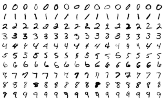
- MNIST dataset
1) 손으로 쓰여진 0부터 9까지의 숫자 이미지들로 구성
2) 흑백 이미지, 모양 = (28, 28)
3) 전체 데이터 셋 = train data 60,000개 + test data 10,000개
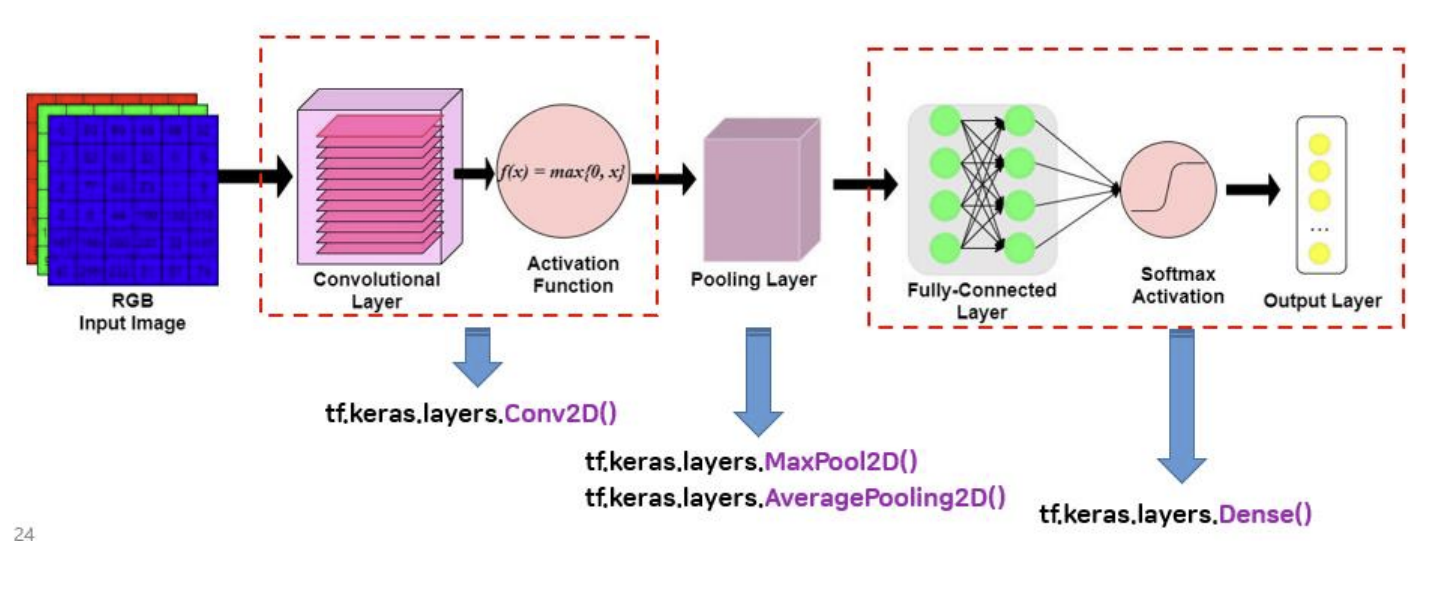
- CNN 모델 구성 소개
Conv2D() 함수
- 용도 : 컨볼루션 계층을 생성하는 함수
- 필요한 라이브러리 임폴트
import tensorflow as tf- 생성 함수 호출
tf.keras.layers.Conv2D(하이퍼파라미터 설정)
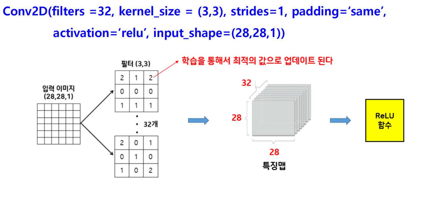
Conv2D() 함수 하이퍼파라미터 설정하기
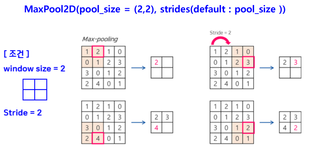
MaxPool2D() 함수
- 용도 : Max Pooling을 수행하는 함수
- 필요한 라이브러리 임폴트
import tensorflow as tf- 생성 함수 호출
tf.keras.layers.MaxPooling2D(하이퍼파라미터 설정)
MaxPool2D() 함수 하이퍼파라미터 설정하기
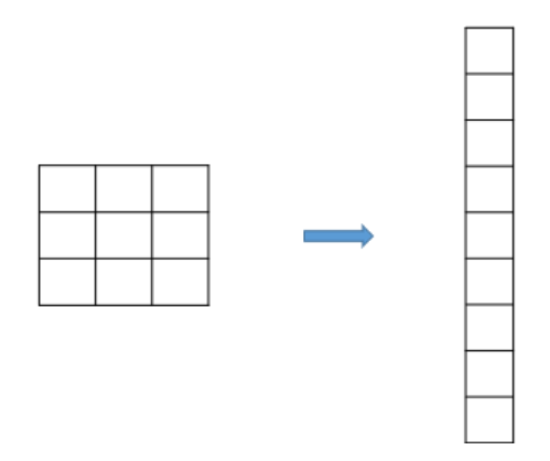
Flatten() 함수
- 용도 : feature map을 1차원 배열로 변환하는 함수
- 필요한 라이브러리 임폴트
import tensorflow as tf- 생성 함수 호출
tf.keras.layers.Flatten()
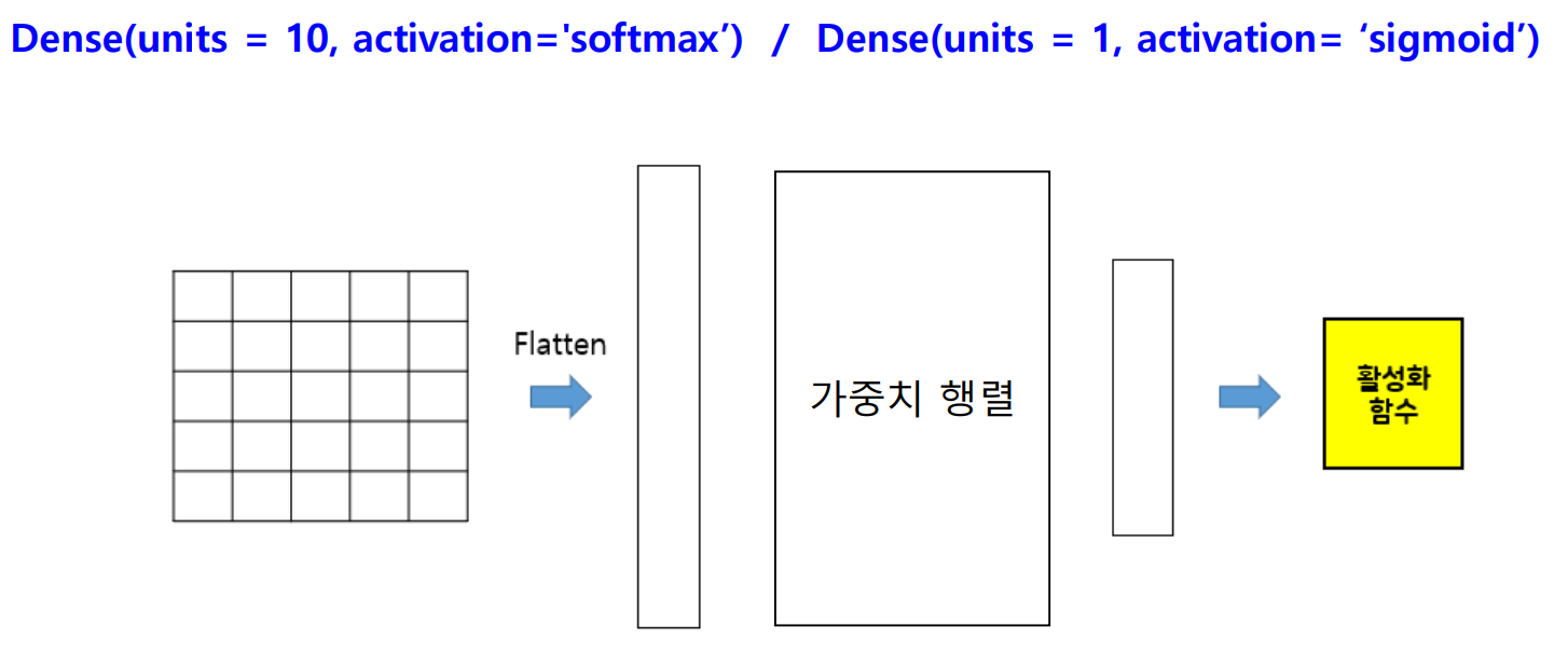
Dense() 함수
- 용도 : 완전 연결 계층(fc layer)을 생성하는 함수
- 필요한 라이브러리 임폴트
import tensorflow as tf- 생성 함수 호출
tf.keras.layers.Dense(하이퍼파라미터 설정)
Dense() 함수 하이퍼파라미터 설정하기
데이터 전처리
1. MNIST dataset 생성하기
- 필요한 라이브러리 임폴트
import tensorflow as tf- MNIST dataset 제공 함수 호출, 다운로드 실행
(X_train, y_train), (X_test, y_test) = tf.keras.datasets.mnist.load_data()
2. 데이터 전처리(1) : 손글씨 이미지 모양 변경
- 기존 shape : (28, 28)
- 변경 후 shape : (28, 28, 1) → 깊이 축 생성, 3차원 형태로 재구성
- np.expand_dims() 함수를 사용
1) np.expand_dims(X_train, axis=-1)
2) np.expand_dims(X_test, axis=-1)
3. 데이터 전처리(2) : normalizing pixel values of an image
- 이미지의 픽셀 값을 0과 1사이로 변경
1) 이미지 : 0 ~ 255 사이의 숫자로 존재
2) 문제점 : 숫자 크기의 차이로 인해서 학습 시 왜곡이 발생
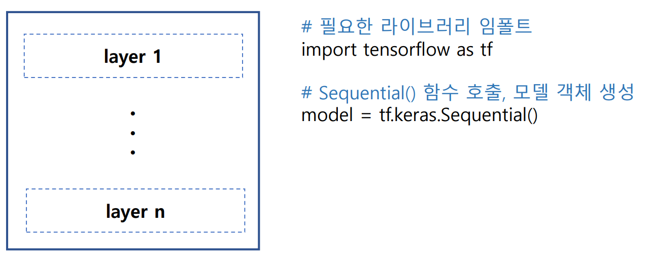
CNN 모델 생성
- Sequential() 함수 : 여러 개의 계층(layer)을 순차적으로 쌓을 수 있는 빈 껍질(컨테이너) 생성
- add() 함수를 이용하여 레이어 추가 → model.add(매개변수 = layer)
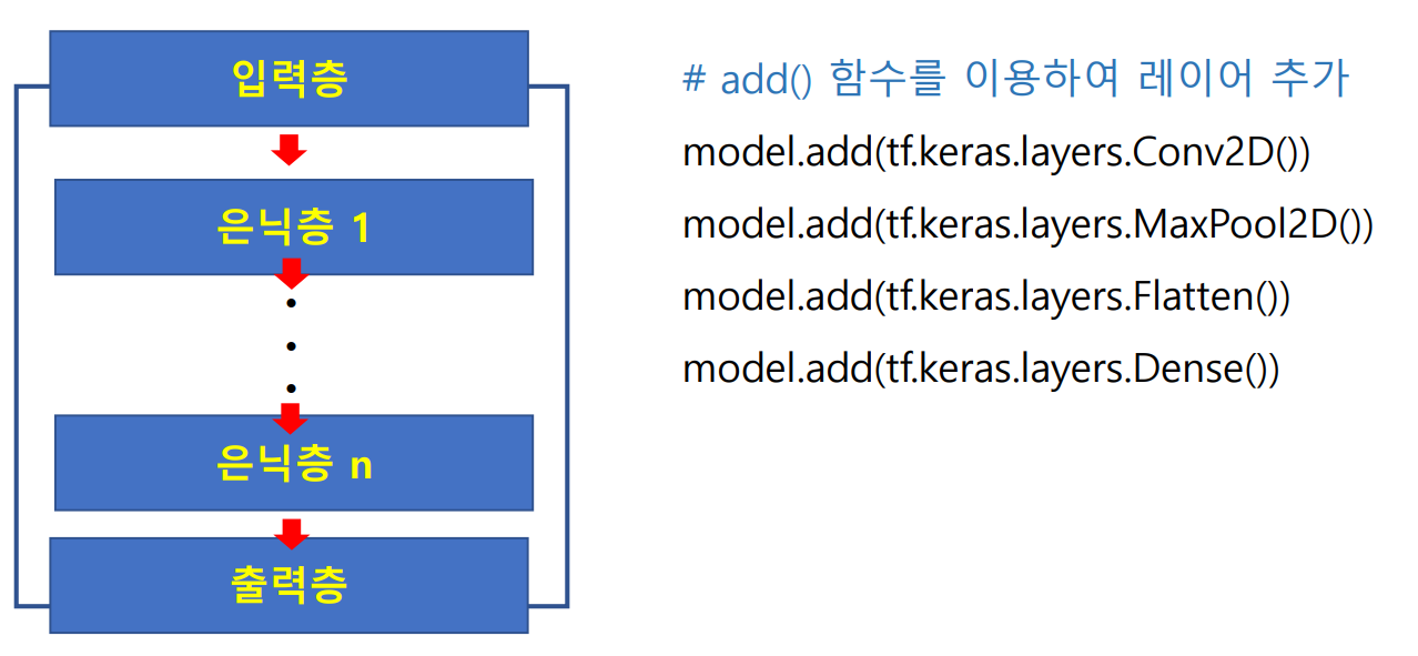
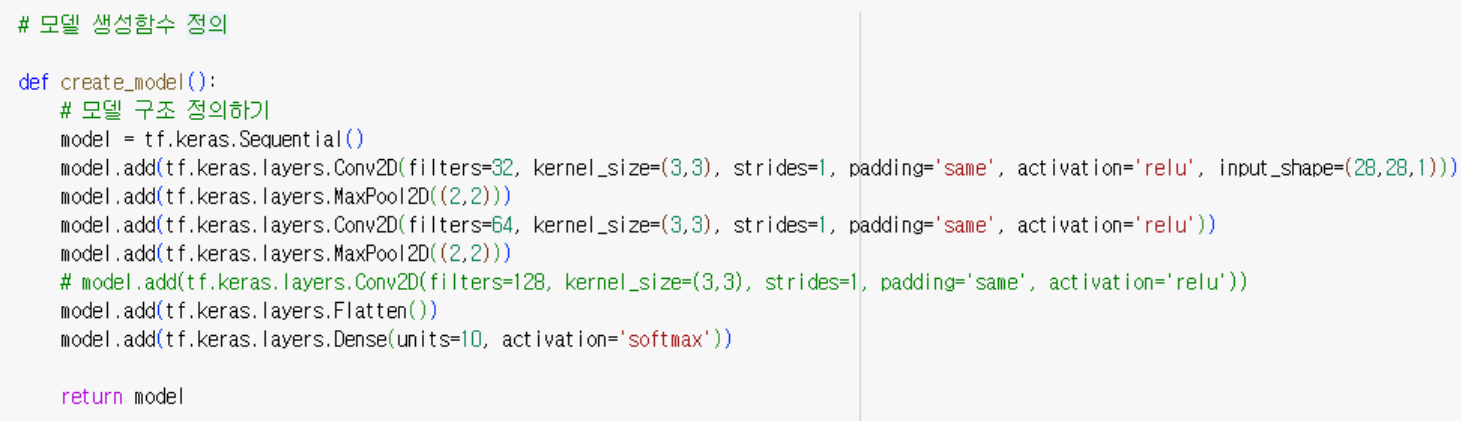
- 모델 생성함수 정의
model 컴파일(compile)
- 개념 : 손실 함수 정의 + 최적화 함수 → 모델 완성
- 손실 함수(loss) : 모델이 계산한 예측과 정답(label)을 비교하여 손실(loss)을 계산
- 최적화 함수(optimizer) : 모델의 가중치를 업데이트하여 손실을 최소화하는 함수
- 학습 : 손실을 최소화하는 가중치 획득 과정

모델 학습
손실 함수(loss function)
- 손실 : 실제 데이터와 모델 예측과의 차이
- 손실의 발생 원인 : 가중치가 최적의 값이 아닐 경우 모델의 예측은 실제 값과 차이가 발생하게 됨
- 손실 함수 : 실제 데이터와 모델 예측과의 차이를 나타내는 수식
손실 함수의 종류
- 이진 분류(binary classification) : tf.keras.losses.BinaryCrossentropy
- model.compile(loss='binary_crossentropy')
- 다중 분류(multi classification)
- tf.keras.losses.CategoricalCrossentropy() : label → One-Hot encoding
- model.compile(loss=‘categorical_crossentropy')
- tf.keras.losses.SparseCategoricalCrossentropy() : label → 정수 인코딩
- model.compile(loss=‘sparse_categorical_crossentropy’)
- 평균 제곱 오차 (MSE)
- 회귀 문제에서 주로 사용
- 예측 값과 실제 값의 제곱 평균 오차를 계산
손실 함수에 대한 이해 : tf.keras.losses.BinaryCrossentropy
- 수식
- H(y, p) : 손실 값
- y : 실제 레이블 (0 또는 1)
- p : 예측값 (시그모이드 함수를 통해 0과 1 사이의 실수값으로 변환된 값)
- 손실 값 계산 예시
- test 데이터 : 실제 레이블이 1이고 모델이 예측한 값이 0.8이라고 가정
- y = 1, p = 0.8
- 손실 값 : H(1, 0.8) = - 1 log(0.8) - (1 - 1) log(1 - 0.8) ≈ 0.313
- 손실 함수 그래프 모양

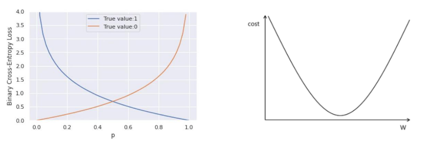
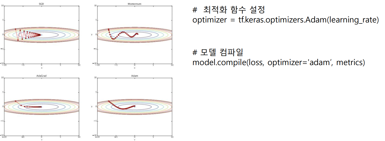
최적화 함수(optimizer)
- 최적화 : 손실 함수의 값이 최소화되도록 가중치를 개선하는 것
- 최적화 함수
1) 최적화 방법을 표현하는 수식
2) 기본 : 경사 하강법
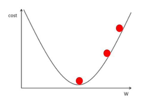
개선된 가중치 = 현재 가중치 – (learning_rate X 현재 가중치에서의 경사(기울기))
최적화 함수의 종류
(이 시리즈의 모든 코드는 코랩환경에서 Python으로 작성하였습니다)
손글씨 이미지를 분류 모델 Code 1 (데이터 생성)
# 필요한 라이브러리 임폴트
import tensorflow as tf
import numpy as np
import matplotlib.pyplot as plt
# mnist dataset 다운로드
(x_train, y_train), (x_test, y_test) = tf.keras.datasets.mnist.load_data()# mnist dataset 확인
print(x_train.shape)
print(y_train.shape)
print(x_test.shape)
print(y_test.shape)
# 학습용 데이터 추출
sample = x_train[0,:,:]
#print(sample)
answer = y_train[0] # 정답 데이터 추출
print(answer)
# 이미지 확인
plt.imshow(sample, cmap='gray')- 이미지 1개 > (H,W,C)
- 이미지 n개 > (N, H, W) - n은 data, 2차원 데이터(흑백 데이터)에 경우
- 3차원 데이터의 경우 (N, H, W, C)
손글씨 이미지를 분류 모델 Code 2 (데이터 전처리)
# 데이터 전처리 1
'''
1. np.expand_dims(data, axis=-1) 함수를 사용
2. 손글씨 이미지의 모양 변경 : 2차원(28, 28) --> 3차원(28, 28, 1)
'''

x_train = np.expand_dims(x_train, axis= -1)
x_test = np.expand_dims(x_test, axis= -1)

# 결과 확인
print(x_train.shape)
print(x_test.shape)
# 데이터 전처리 2
'''
1. normalization 실행
2. 이미지의 픽셀 값을 0과 1사이로 변경 --> 필수!!!
'''
x_train = x_train / 255
x_test = x_test / 255
# 결과 확인
print(np.max(x_train[0,:,:,:]))
print(np.min(x_train[0,:,:,:]))
print('-'*100)
print(np.max(x_test[0,:,:,:]))
print(np.min(x_test[0,:,:,:]))# 필요한 함수 임폴트
from sklearn.model_selection import train_test_split
'''
1. train_test_split() 함수를 사용
2. 학습용 데이터의 일부를 검증용 데이터로 분할
'''
x_train, x_val, y_train, y_val = train_test_split(x_train, y_train, test_size=0.2, random_state=0)
# 결과 확인
print(x_train.shape)
print(x_val.shape)
print(y_train.shape)
print(y_val.shape)- 데이터 전처리 : normalizing pixel values of an image
- 이미지의 픽셀 값을 0과 1사이로 변경
- 이미지 : 0 ~ 255 사이의 숫자로 존재
- 문제점 : 숫자 크기의 차이로 인해서 학습 시 왜곡이 발생
- 이미지의 픽셀 값을 0과 1사이로 변경
손글씨 이미지를 분류 모델 Code 3 (학습용 / 검증용 데이터 생성)
# 필요한 함수 임폴트
from sklearn.model_selection import train_test_split

'''
1. train_test_split() 함수를 사용
2. 학습용 데이터의 일부를 검증용 데이터로 분할
'''

x_train, x_val, y_train, y_val = train_test_split(x_train, y_train, test_size=0.2, random_state=0)

# 결과 확인
print(x_train.shape)
print(x_val.shape)
print(y_train.shape)
print(y_val.shape)
손글씨 이미지를 분류 모델 Code 4 (CNN 모델 생성)
# 모델 생성 함수 정의

def create_model():
  model = tf.keras.Sequential()

  model.add(tf.keras.layers.Conv2D(
      filters=32,
      kernel_size=(3,3),
      strides=1,
      padding='same',
      activation='relu',
      input_shape=(28,28,1)
      )
  )

  model.add(tf.keras.layers.MaxPool2D(pool_size=(2,2)))

  model.add(tf.keras.layers.Conv2D(
      filters=64,
      kernel_size=(3,3),
      strides=1,
      padding='same',
      activation='relu',
      )
  )

  model.add(tf.keras.layers.MaxPool2D(pool_size=(2,2)))

  model.add(tf.keras.layers.Flatten())

  model.add(tf.keras.layers.Dense(units=10, activation='softmax'))

  return model

# 모델 생성
model = create_model()
# 모델 구조
model.summary()# model compile : 손실함수, 최적화 함수 > 모델 완성
model.compile(
loss='sparse_categorical_crossentropy',
optimizer='adam',
metrics=['accuracy']
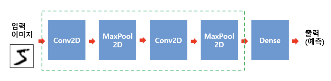
)- CNN hidden layer
- Conv2D > MaxPool2D > Conv2D > MaxPool2D > flatten
손글씨 이미지를 분류 모델 Code 5 (CNN 모델 학습 및 평가)
# 모델 학습

history = model.fit(
    x = x_train,
    y = y_train,
    batch_size = 128,
    epochs=20,
    validation_data = (x_val, y_val)
)
# 학습의 결과물 저장 변수 history
print(history.history)
print(type(history.history))# 학습결과 시각화 - 검증용 데이터
#직선 그래프
plt.plot(history.history['val_accuracy'], label='val_accuracy')
plt.plot(history.history['accuracy'], label='accuracy')
plt.legend()
plt.show()
plt.plot(history.history['val_loss'], label='val_loss')
plt.plot(history.history['loss'], label='loss')
plt.legend()
plt.show()# 평가용 데이터 전체에 대한 성능 평가
result = model.evaluate(x = x_test, y = y_test, batch_size = 100)
print(result)참고 자료

AI & Robotics