github : https://github.com/nalinzip/ml_study

colab : https://colab.research.google.com/drive/14wzHk55v1fJU9m14VuAjW5DaAiyM7-_M?usp=sharing

1. 사이킷런 (scikit-learn) 특징

• 머신러닝 라이브러리 -> 가장 쉽고 효율적인 개발 라이브러리, 프레임워크와 API 를 제공

버전 확인법

import sklearn
print(sklearn.__version__)

2. 첫 번째 머신러닝 만들어 보기 - 붓꽃 품종 예측하기

데이터 세트로 붓꽃의 품종을 분류(Classification)하는 것입니다.

• 분류 같은 지도학습은 학습을 위한 다양한 피처와 분류 결정값인 레이블 (Label) 데이터로 모델을 학습한 뒤 , 별도의 테스트 데이터 세트에서 미지의 레이블을 예측합니다.

from sklearn.datasets import load_iris
from sklearn.tree import DecisionTreeClassifier
from sklearn.model_selection import train_test_split

• 사이킷런 패키지 내의 모듈명은 sklearn 으로 시작함
• sklearn.datasets = 자체적으로 제공하는 세트를 생성하는 모듈의 모임
• sklearn.model_selection = 학습 데이터와 검증 데이터 , 예측 데이터로 데이터를 분리하거나 최적의 하이퍼 파라미터로 평가하기 위한 다양한 모듈
  의 모임
• train_test_split() = 데이터 세트를 학습 데이터와 테스트 데이터로 분리하는 데 사용하는 함수

- 하이퍼 파라미터란

• 머신러닝 알고리즘별로 최적의 학습을 위해 직접 입력하는 파라미터들을 통칭
• 하이퍼 파라미터를 통해 머신러닝 알고리즘의 성능을 튜닝할 수 있음.

import pandas as pd
# 붓꽃 데이터 세트를 로딩합니다.
iris = load_iris()
# iris.data는 Iris 데이터 세트에서 피처(feature)만으로 된 데이터를 numpy 로 가지고 있습니다.
iris_data = iris.data
#iris.target은 붓꽃 데이터 세트에서 레이블 ( 결정 값 ) 데이터를 numpy 로 가지고 있습니다.
iris_label = iris. target
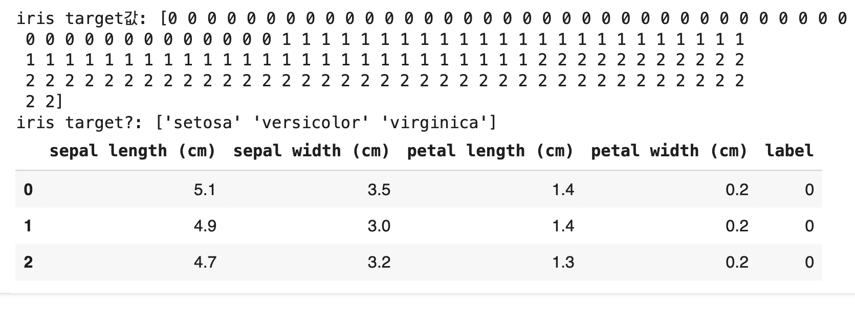
print('iris target값:', iris_label)
print('iris target?:', iris.target_names)
# 붓꽃 데이터 세트를 자세히 보기 위해 DataFrame 으로 변환합니다.
iris_df = pd.DataFrame(data=iris_data, columns=iris.feature_names)
iris_df[ 'label'] = iris. target
iris_df.head (3)

load_iris() 함수

• 붓꽃 데이터 세트를 로딩한 후 , 피처들 (sepal length, sepal width, petal length, petal width 가)과 데이터 값이 어떻게 구성되어 있는지를 확인하기 위해 DataFrame 으로 변환.

• 레이블 (결정값) 은 0, 1, 2

• 0 = Setosa 품종

• 1 이 versicolor 품종

• 2 가 vinginica 품종

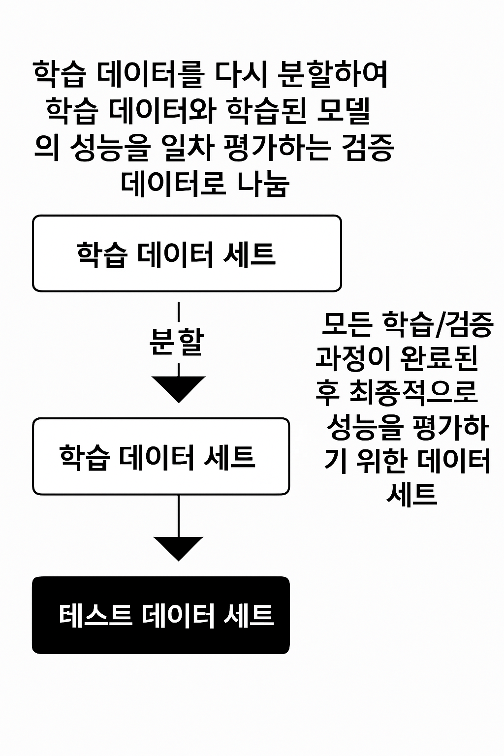
학습용 데이터와 테스트용 데이터는 반드시 분리해야 함!!!!

• 학습 데이터로 학습된 모델이 얼마나 뛰어난 성능을 가지는지 평가하려면 테스트 데이터 세트가 필요하기 때문임.
• train_test_split() API 제공되어 있음
• test_size 파라미터 입력값의 비율
  로 쉽게 분할

X_train, X_test, y_train, y_test = train_test_split(iris_data, iris_label,
                                                    test_size=0.2, random_state=11)

파라미터

• iris_data : 피처 데이터 세트
• iris_label : 레이블 (Label) 데이터 세트
• test_size = 0.2 : 전체 데이터 세트 중 테스트
  데이터 세트의 비율
  예) 전체 데이터가 20%, 학습 데이터가 80% 로 데이터를 분할하기
• random_state : 호출할 때마다 같은 학습/테스트 용 데이터 세트를 생성하기 위해 주어지는 난수 발생 값

(random_state 는 random값을 만드는 seed와 같은 의미. 숫자 자체는 어떤 값을 지정해도 상관없음)

머신러닝 분류 알고리즘의 하나인 의사 결정 트리

# DecisionTreeClassifier 객체 생성
dt_clf = DecisionTreeClassifier(random_state=11)
# 학습 수행
dt_clf.fit(X_train, y_train)![](https://velog.velcdn.com/images/nunnalin/post/d68ffb68-23e0-4622-96fd-853c9288f95c/image.png)

사이킷런의 의사 결정 트리 클래스

- DecisionTreeClassifier를 객체로 생성 (random_state=11 : 동일한 학습 / 예측 결과를 출력하기 위한 용도로만 사용)

• 생성된 DecisionTreeClassifier 객체의 fit() 메서드에 학습용 피처 데이터 속성과 결정값 데이터 세트를 입력해 호출하면 학습을 수행

# 학습이 완료된 DecisionTreeclassifier 객체에서 테스트 데이터 세트로 예측 수행.
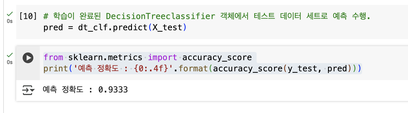
pred = dt_clf.predict(X_test)

• predict() 메서드에 테스트용 피처 데이터 세트를 입력해 호출하면 학습된 모델 기반에서 테스트 데이터 세트에 대한 예측값을 반환함

• 정확도 측정을 위해 accuracy_score() 함수
• 측, 정확도가 약 0.9333(93.33%) 으로 측정

예측 프로세스 정리

1.데이터 세트 분리 : 데이터를 학습 데이터 vs 테스트 데이터로 분리.
2.모델 학습 : 학습 데이터를 기반으로 ML 알고리즘을 적용해 모델을 학습시킴.
3.예측 수행 : 학습된 ML 모델을 이용해 테스트 데이터의 분류 (즉, 붓꽃 종류) 를 예측.
4.평가 : 이렇게 예측된 결값과 테스트 데이터의 실제 결값을 비교해 ML 모델 성능을 평가.

3. 사이킷런의 기반 프레임워크 익히기

Estimator 이해 및 fit(), predict() 메서드

• Estimator : 지도학습 (Classifier 와 Regressor)의 모든 알고리즘을 구현한 클래스
• Estimator 내부에서 fit()& predict()
• fit() : ML 모델 학습을 위해서
• predict() : ML 모델의 예측을 위해 predict()
• Estimator 의 fit()과 predict()를 호출해서 평가를 하거나 하이퍼 파라미터 튜닝을 수행하는 것
  -fit() 은 지도학습의 fit() 과 같이 학습을 의미하는 것이 아니라 입력 데이터의 형태에 맞춰 데이터를 변환하기 위한 사전 구조를 맞추는 작업

사이킷런의 주요 모듈

예제 데이터

• sklearn.datasets : 사이킷런에 내장되어 예제로 제공하는 데이터 세트

피처 처리

• sklearn.preprocessing : 데이터 전처리에 필요한 다양한 가공 기능 제공 (문자열을 숫자
  형 코드 값으로 인코딩. 정규화, 스케일링 등)
• sklearn.feature_selection : 알고리즘에 큰 영향을 미치는 피처를 우선순위대로 셀렉션 작
  업을 수행하는 다양한 기능 제공
• sklearn.feature_extraction : 텍스트 데이터나 이미지 데이터의 벡터화된 피처를 추출하는 데 사용됨.

피치 처리 & 차원 축소

• sklearn.decomposition : 차원 축소와 관련한 알고리즘을 지원하는 모듈임. PCA, NMF.
  Truncated SVD 등을 통해 차원 축소 기능을 수행할 수 있음

데이터 분리, 검증 & 파라미터

• sklearn.model_selection

평가

• sklearn.metrics

ML 알고리즘

• sklearn.ensemble
• sklearn.linear_model
• sklearn.naive_bayes
• sklearn.neighbors
• sklearn.svm
• sklearn.tree
• sklearn.cluster

유틸리티

• sklearn.pipeline

머신러닝 모델을 구축하는 주요 프로세스는

• 피처의 가공
• 변경
• 추출을 수행하는 피처 처리 (feature processing)
• ML 알고리즘 학습/예측 수행
• 모델 평가의 계를 반복적으로 수행

내장된 예제 데이터 세트

• 데이터는 datasets 모듈에 있는 여러 API 를 호출해 만들 수 있음
• datasets.load_boston()
• datasets.load_breast_cancer()
• datasets.load_diabetes()
• datasets.load_digits()
• datasets.load_iris()

fetch 계열의 명령

인터넷에서 내려받아 홈 디렉터리 아래의 scikit learn_data라는 서브 디렉터리에 저장한 후 추후 불러들이는 데이터임
인터넷 연결해야 사용할 수 있음

• fetchcovtype(): 회귀 분석용 토지 조사 자료
• fetch_20newsgroups(): 뉴스 그룹 텍스트 자료
• fetch_olivetti_faces(): 얼굴 이미지 자료
• fetch_lfw_people(): 얼굴 이미지 자료
• fetch_lfw_pairs(): 얼굴 이미지 자료
• fetch_ccv1(): 로이터 뉴스 말뭉치
• fetch_mldata(): ML 웹사이트에서 다운로드

분류와 클러스터링을 위한 표본 데이터 생성기

• datasets.make_classifications( ) : 분류를 위한 데이터 세트를 만듭니다. 특히 높은 상관도 , 불필요한 속성 등의 노이즈 효과를 위한 데이터를 무작위로 생성해줌.

• datasets.make_blobs( ) : 클러스터링을 위한 데이터 세트를 무작위로 생성해줌.

사이킷런에 내
장된 이 데이터 세트는 일반적으로 딕셔너리 형태로 돼 있습니다.

키

• data : 피처의 데이터 세트를 가리킴
• target : 분류 시 레이블 값 , 회귀일 때는 숫자 결괏값 데이터 세트
• target_names : 개별 레이블의 이름을 나타냄.
• teature_names : 피처의 이름을 나타냄.
• DESCR : 데이터 세트에 대한 설명과 각 피처의 설명을 나타냄.

from sklearn.datasets import load_iris
iris_data = load_iris()
print(type(iris_data))

• load_iris() API 의 반환 결과는 sklearn.utils,Bunch 클래스

keys = iris_data.keys()
print('붓꽃 데이터 세트의 키들 :', keys)

출력은 아래와 같이 나옴

붓꽃 데이터 세트의 키들 : dict_keys(['data', 'target', 'frame', 'target_names', 'DESCR', 'feature_names', 'filename', 'data_module'])

print('\n feature_names 의 type:', type(iris_data.feature_names))
print('feature_names 의 shape:', len(iris_data.feature_names))
print(iris_data.feature_names)
print('\n target_names 의 type:', type(iris_data.target_names))

print('target_names 의 shape:', len(iris_data. target_names))
print(iris_data.target_names)
print('\n data 의 type:', type(iris_data.data))
print(' data 의 shape:', iris_data.data.shape)
print(iris_data[ 'data'])
print('\n target 의 type:', type(iris_data.target))
print('target 의 shape:'
, iris_data. target.shape)
print(iris_data.target)

출력은 아래와 같이 나옴

feature_names 9 type: (class 'list'>
feature_names 9 shape: 4
['sepal length (cm)', 'sepal width (cm)', 'petal length (cm)', 'petal width (cm) ']
target_names © type: (class 'numpy.ndarray'>
target_names ® shape: 3
['setosa' 'versicolor' 'virginica']
data 9 type: (class 'numpy.ndarray'>
data ° shape: (150, 4)
[[5.1 3.5 1.4 0.2]
[4.9 3. 1.4 0.2]
[6.5 3. 5.2 2. ]
[6.2 3.4 5.4 2.3]
[5.9 3. 5.1 1.8]1
target © type: <class 'numpy.ndarray'>
target © shape: (150, )
1 0 0 0 0 0 0 0 0 0 0 0 0 0 0 0 0 0 0 0 0 0 0 0 0 0 0 0 0 0 0 0 0 0 0 0 0
0 0 0 0 0 0 0 0 0 0 0 0 0 1 8 1 1 1 1 1 1 1 1 1 1 1 1 1 1 1 1 1 1 1 1 1
1 1 1 1 1 1 1 1 1 1 1 1 1 1 1 1 1 1 1 1 1 1 1 1 1 1 2 2 2 2 2 2 2 2 2 2 2
2 2 2 2 2 2 2 2 2 2 2 2 2 2 2 2 2 2 2 2 2 2 2 2 2 2 2 2 2 2 2 2 2 2 2 2 2
2 2]

4. Model Selection 모듈 소개

model_selection 모듈란

• 학습 데이터와 테스트 데이터 세트를 분리하거나 교차 검증 분
  할 및 평가 그리고 Estimator의 하이퍼 파라미터를 튜닝하기 위한 다양한 함수와 클래스를 제공하는 모듈임.

학습 / 테스트 데이터 세트 분리 - train_test_split)

from sklearn.metrics import accuracy_score
iris = load_iris()
dt_clf = DecisionTreeClassifier()
train_data = iris.data
train_label = iris.target
dt_clf. fit(train_data, train_label)
# 학습 데이터 세트으로 예측 수행
pred = dt_clf.predict(train_data)
print(' 예측 정확도 :', accuracy_score(train_label, pred))

결과

예측 정확도 : 1.0

• 이미 학습한 학습 데이터 세트를 기반으로 예측했기 때문에 예측 정확도 100% 나오는 경우가 있음.

• 따라서 전용의 테스트 데이터 세트여야 함.

• sklearn.model_selection 모듈에서 train_test_split() 를 통해 쉽게 분리할 수 있음

• train_test_split()는 첫 번째 파라미터로 피처 데이터 세트, 두 번째 파라미터로 레이블 데이터 세트를 입력받음.

• 그리고 선택적으로 다음 파라미터를 입력받음.

• test_size: 전체 데이터에서 테스트 데이터 세트 크기를 얼마로 샘플링할 것인가를 결정함.
  디폴트는 0.25, 즉 25% 임.

• train_size: 전체 데이터에서 학습용 데이터 세트 크기를 얼마로 샘플링할 것인가를 결정함.
  텍스트_test_size parameter를 통상적으로 사용하기 때문에 train_size 는 잘 사용되지 않음.

• shuffle: 데이터를 분리하기 전에 데이터를 미리 섞을지를 결정함.
  디폴트는 True 입니다. 데이터를 분산시켜서 좀 더
  효율적인 학습 및 테스트 데이터 세트를 만드는 데 사용됩니다.

• random_state: random_state는 호출할 때마다 동일한 학습/테스트용 데이터 세트를 생성하기 위해 주어지는 난수 값임.

train_test_split( )는 호출 시 무작위로 데이터를 분리하므로 random_state 를 지정하지 않으면 수행할 때마다 다른
학습 / 테스트 용 데이터를 생성함.

• train_test_split() 의 반환값은 튜플 형태입니다.
  순차적으로 학습용 데이터의 피처 데이터 세트 , 테스트용 데이터의 피처 데이터 세트, 학습용 데이터의 레이블 데이터 세트, 테스트용 데이터의 레이블 데이터 세트가 반환됩니다.

붓꽃 데이터 세트를 train_test_split()을 이용해서 나누어져 있음

• 테스트 데이터 세트를 전체의 30%
• 학습 데이터 세트를 나머지 70%

from sklearn. tree import DecisionTreeClassifier
from sklearn.metrics import accuracy_score
from sklearn.datasets import load_iris
from sklearn.model_selection import train_test_split
dt_clf = DecisionTreeClassifier()
iris_data = load_iris( )
X_train, X_test, y_train, y_test = train_test_split(iris_data.data, iris_data.target, \
                                                    test_size=0.3, random_state=121)

dt_clf.fit(X_train, y_train)
pred = dt_clf.predict(X_test)
print('예측 정확도 : {0: 4f}'.format(accuracy_score(y_test, pred)))

예측 정확도 :  0.955556

• 테스트 데이터로 예측을 수행한 결과 정확도가 약 95.56%라는 뜻
• 데이터 양이 크지 않아 알고리즘의 예측 성능을 판단하기에는 그리 적절하지 않습니다.
• 학습을 위한 데이터의 양을 일정 수준 이상으로 보장하는 것도 중요하지만, 학습된 모델에 대해 다양한 데이터를 기반으로 예측 성능을 평가해보는 것도 매우 중요

교차 검증

알고리즘을 학습시키는 학습 데이터와 이에 대한 예측 성능을 평가하기 위한 별도의 테스트용 데이터가 필요하지만 과적합 (Overfitting) 에 취약한 약점을 가질 수 있음

• 학습 데이터에만 과도하게 최적화되어 -> 실제로 예측 시 예측 성능이 과도하게 떨어짐!

• 일반화된 성능을 갖춘 모델을 만드는 것이 중요.

• 교차 검증은 이러한 데이터 편중을 막기 위해서 별도의 여러 세트로 구성된 학습 데이터 세트와 검증 데이터 세트에서 학습과 평가를 수행하는 것임.

• 각 세트에서 수행한 평가 결과에 따라 하이퍼 파라미터 튜닝 등의 모델 최적화를 더욱 손쉽게 할 수 있음.

• 대부분의 ML 모델의 성능 평가는 교차 검증 기반으로 1차 평가를 한 뒤에 최종적으로 테스트 데이터 세트에 적용해 평가하는 프로세스임.

- ML에 사용되는 데이터 세트를 세분화

1. 학습
2. 검증
3. 테스트

K 폴드 교차 검증

• K 폴드 교차 검증은 가장 보편적으로 사용되는 교차 검증 기법임.
• 먼저 K 개의 데이터 폴드 세트를 만들어서 K 번만큼 각 폴트 세트에 학습과 검증 평가를 반복적으로 수행하는 방법임.
• 다음 그림은 5 폴드 교차 검증을 수행 (즉, K 가 5).

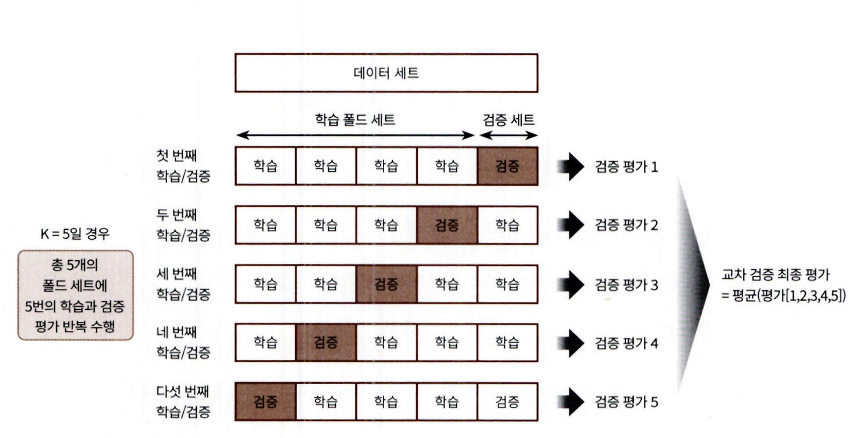
1. 5개의 폴드된 데이터 세트를 학습과 검증을 위한 데이터 세트로 변경하면서 5번 평가를 수행
2. 5개의 평가를 평균한 결과를 가지고 예측 성능을 평가

• 데이터 세트를 K 등분 (5등분) 합니다.

• 첫 번째 반복에서는 처음부터 4개 등분을 학습 데이터 세트

• 마지막 5번째 등분 하나를 검증 데이터 세트로 설정하고 학습 데이터 세트에서 학습 수행, 검증 데이터 세트에서 평가를 수행

• 첫 번째 평가를 수행하고 나면 이제 두 번째 반복에서 다시 비슷한 학습과 평가 작업을 수행

• 단, 이번에는 학습 데이터와 검증 데이터를 변경
  (처음부터 3개 등분까지, 그리고 마지막 5번째 등분을 학습 데이터 세트로, 4번째 등분 하나를 검증 데이터 세트로 설정).

• 이렇게 학습 데이터 세트와 검증 데이터 세트를 점진적으로 변경하면서b 마지막 5 번째 (K 번째) 까지 학습과 검증을 수행하는 것이 바로 K 폴드 교차 검증입니다.

• 5개 (K 개) 의 예측 평가를 구했으면 이를 평균해서 K 폴드 평가 결과로 반영하면 됩니다.

• 사이킷런에서는 K 폴드 교차 검증 프로세스를 구현하기 위해
  KFold와 StratifiedKFold 클래스를 제공합니다.

• 먼저 KFold 클래스를 이용해 붓꽃 데이터 세트를 교차 검증하고 예측 정확도를 알아보겠습니다.

• 붓꽃 데이터 세트와 DecisionTreeClassifier 를 다시 생성합니다. 그리고 5 개의 폴드 세트로 분리하는 KFold 객체를 생성합니다.

from sklearn.tree import DecisionTreeClassifier
from sklearn.metrics import accuracy_score
from sklearn.model_selection import KFold
import numpy as np
iris = load_iris()
features = iris.data
label = iris.target
dt_clf = DecisionTreeClassifier(random_state=156)
kfold = KFold(n_splits=5)
cv_accuracy = []
print('붓꽃 데이터 세트 크기 :', features.shape [0])

# 붓꽃 데이터 세트 크기 : 150 출력

n_iter = 0
cv_accuracy = []

# KFold 객체의 split()를 호출하면 폴드별 학습용, 검증용 테스트의 로우 인덱스를 array로 반환
for train_index, test_index in kfold.split(features):
    # kfold.split()으로 반환된 인덱스를 이용해 학습용, 검증용 테스트 데이터 추출
    X_train, X_test = features[train_index], features[test_index]
    y_train, y_test = label[train_index], label[test_index]

    # 학습 및 예측
    dt_clf.fit(X_train, y_train)
    pred = dt_clf.predict(X_test)
    n_iter += 1

    # 반복 시마다 정확도 측정
    accuracy = np.round(accuracy_score(y_test, pred), 4)
    train_size = X_train.shape[0]
    test_size = X_test.shape[0]

    # 출력
    print('\n#{} 교차 검증 정확도: {}, 학습 데이터 크기: {}, 검증 데이터 크기: {}'
          .format(n_iter, accuracy, train_size, test_size))
    print('#{} 검증 세트 인덱스: {}'.format(n_iter, test_index))

    cv_accuracy.append(accuracy)

# 평균 검증 정확도 계산
print('\n## 평균 검증 정확도 :', np.mean(cv_accuracy))

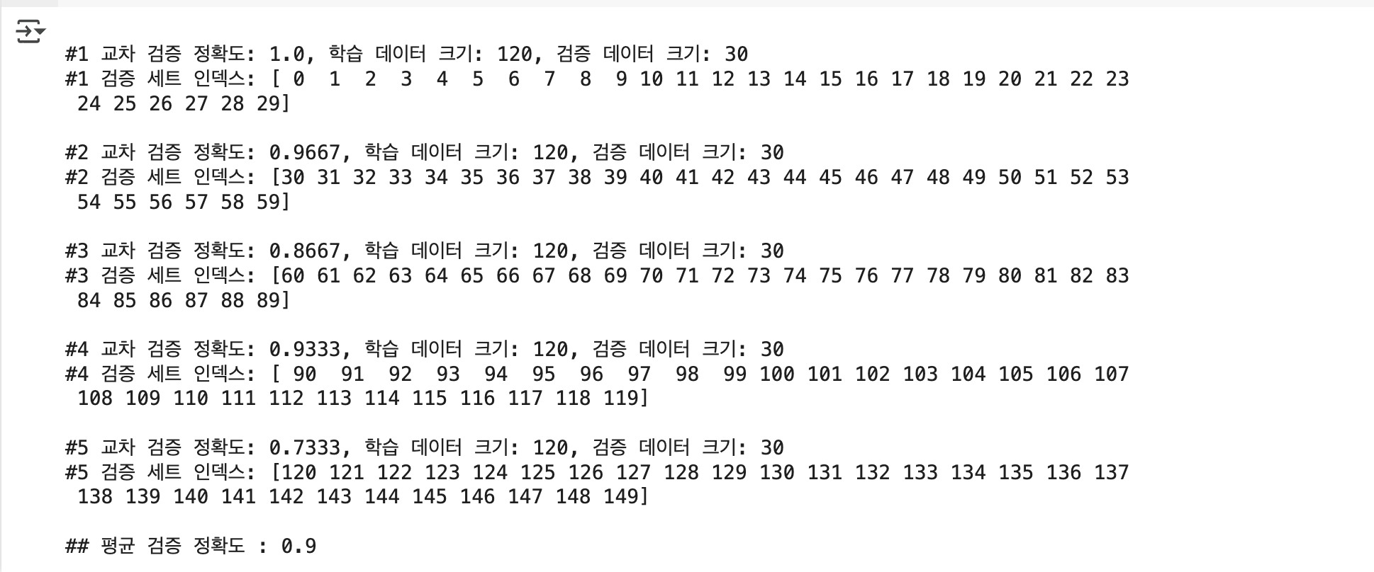
• KFold(n_splits=5)로 KFold 객체를 생성했으니 Split()을 호출해 전체 붓꽃 데이터를 5 개의 폴드 데이터 세트로 분리.

• KFold 객체는 split() 을 호출하면 학습용 / 검증용 데이터로 분할할 수 있는 인덱스를 반환.

• 전체 붓꽃 데이터는 모두 150개 -> 학습용 데이터 세트는 이 중 4/5 인 120 개, 검증 테스트 데이터 세트는 1/5 인 30 개로 분할됨.

• 실제로 학습용 / 검증용 데이터 추출은 반환된 인덱스를 기반으로 개발 코드에서 직접 수행해야 함.

• 본 예제는 5 개의 폴드 세트를 생성하는 KFold 객체의 split()을 호출해 교차 검증 수행 시마다 학습과 검증을 반복해 예측 정확도를 측정함.
  - split() 이 어떤 값을 실제로 반환하는지도 확인해 보기 위해 검증 데이터 세트의 인덱스도 추출.

Stratified K 폴드

• 불균형한 (imbalanced) 분포도를 가진 레이블 ( 결정 클래스 ) 데이터 집합을 위한 K폴드 방식임
• 불균형한 분포도를 가진 레이블 데이터 집합은 특정 레이블 값이 특이하게 많거나 매우 적어서 값의 분포가 한쪽으로 치우치는 것을 말함
• 대출 사기 데이터를 예로 들면, 전체 1억 건 중 대출 사기 1000건이면 0.0001%의 비율
• K 폴드로 랜덤하게 학습 및 테스트 세트 인덱스를 고르면 레이블 값의 비율을 반영하지 못하는 경우가 쉽게 발생함.
• 레이블 값이 1인 데이터가 반복에 따라 많이 포함되거나 아예 없는 세트가 발생할 수 있음.
• Stratified K 폴드는 대출 사기에 대한 문제 해결 가능 : 대출 사기 레이블이 1인 데이터는 비록 건수는 작지만 중요한 피처 값을 가지고 있어서 매우 중요한 데이터임.
• 따라서 원본 데이터와 유사한 레이블 값의 분포를 학습/테스트 세트에도 유지하는 게 매우 중요함.

1. 원본 데이터의 레이블 분포를 고려
2. 이 분포와 동일하게 학습과 검증 데이터 세트를 분배
3. K 폴드가 어떤 문제를 가지고 있는지 확인 (사이킷런의 StratifiedKFold 클래스를 이용)
4. 붓꽃 데이터 세트를 간단하게 DataFrame으로 생성하고 레이블 값의 분포도를 확인.

import pandas as pd
from sklearn.datasets import load_iris
iris = load_iris()
iris_df = pd.DataFrame(data=iris.data, columns=iris.feature_names)
iris_df['label']=iris.target
iris_df['label'].value_counts()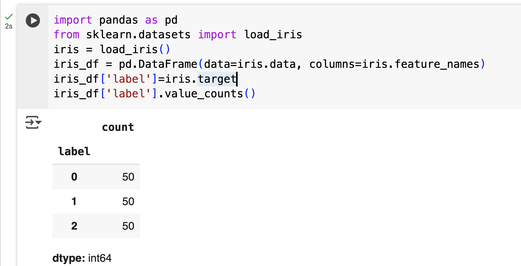

• 레이블 값은 0, 1, 2 값 모두 50 개로 동일.
• 이슈가 발생하는 현상을 도출하기 위해 3개의 폴드 세트를 KFold 로 생성하고 각 교차 검증 시마다 생성되는 학습/검증 레이블 데이터 값의 분포도를 확인 필수.

from sklearn.model_selection import KFold
kfold = KFold(n_splits=3)
n_iter =0
for train_index, test_index in kfold.split(iris_df):
  n_iter += 1
label_train= iris_df ['label'].iloc[train_index]
label_test= iris_df ['label' ].iloc[test_index]
print('# 교차 검증 : {0}'.format(n_iter))
print('학습 레이블 데이터 분포 :Mn', label_train.value_counts())
print(' 검증 레이블 데이터 분포 :M', label_test.value_counts())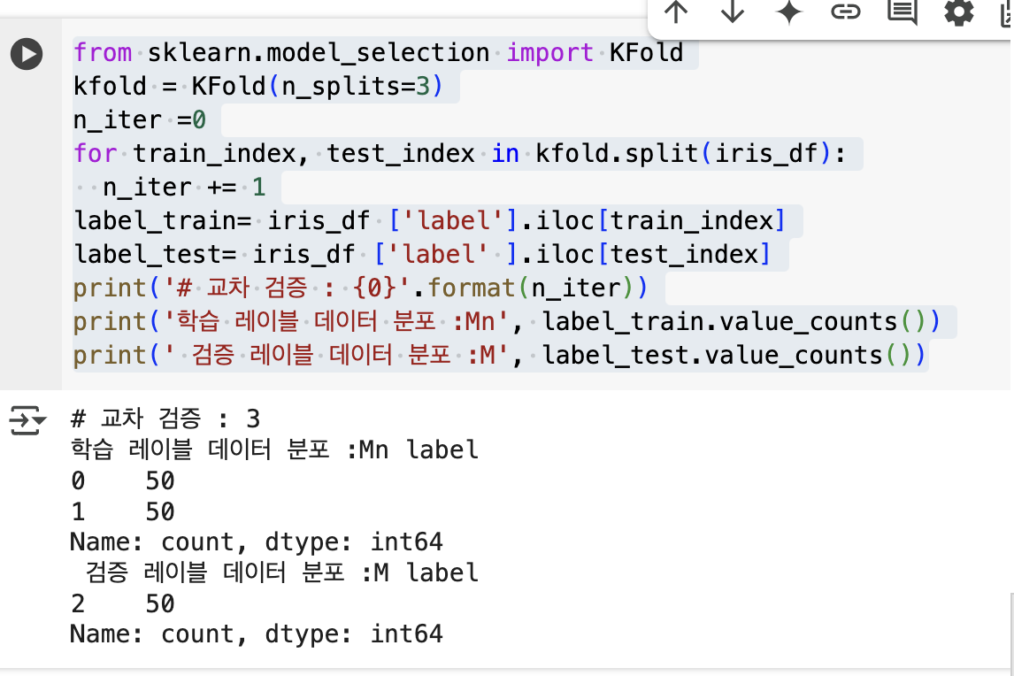

• 교차 검증 시마다 3 개의 폴드 세트로 만들어지는 학습 레이블과 검증 레이블이 완전히 다른 값으로 추출됨.

• 예를 들어 첫 번째 교차 검증에서는 학습 레이블의 1, 2 값이 각각 50 개가 추출되었고, 검증 레이블의 0 값이 50 개 추출되었습니다.

학습 레이블은 1, 2 밖에 없으므로 0 의 경우는 전혀 학습하지 못합니다.

반대로 검증 레이블은 0 밖에 없으므로 학습 모델은 절대 0 을 예측하지 못합니다.

이런 유형으로 교차 검증 데이터 세트를 분할하면 검증 예측 정확도는 0 이 될 수밖에 없습니다.

StratifiedKFold는 이렇게 KFold로 분할된 레이블 데이터 세트가 전체 레이블 값의 분포도를 반영하지 못하는 문제를 해결해 줍니다.

이번에는 동일한 데이터 분할을 StratifiedKFold로 수행하고 학습 / 검증 레이블 데이터의 분포도를 확인해 보겠습니다.

StratifiedKFold 를 사용하는 방법은 KPold 를 사용하는 방법과 거의 비슷합니다.

단 하나 큰 차이는 StratifiedKPold 는 레이블 데이터 분포도에 따라 학습 / 검증 데이터를 나누기 때문에
split() 메서드에 인자로 피처 데이터 세트뿐만 아니라 레이블 데이터 세트도 반드시 필요하다는 사실입니다
(K 폴드의 경우 레이블 데이터 세트는 split() 메서드의 인자로 입력하지 않아도 무방합니다).

폴드 세트는 3 개로 설정하겠습니다.

🌟 중요 포인트 (핵심 강조):
일반 KFold는 레이블 분포를 반영하지 않아 불균형한 학습/검증 세트가 생성될 수 있음

학습 레이블에 특정 클래스가 없으면, 모델은 그 클래스를 학습하지 못하고 예측 정확도 0 발생

StratifiedKFold는 이러한 문제를 해결하고, 레이블 분포를 유지하며 학습/검증 세트를 나눔

StratifiedKFold 사용 시 split()에 레이블도 반드시 함께 전달해야 함

폴드 수는 이 예제에서는 3 개로 설정됨

일반 KFold는 레이블 분포를 반영하지 않아 불균형한 학습/검증 세트가 생성될 수 있음

학습 레이블에 특정 클래스가 없으면, 모델은 그 클래스를 학습하지 못하고 예측 정확도 0 발생

StratifiedKFold는 이러한 문제를 해결하고, 레이블 분포를 유지하며 학습/검증 세트를 나눔

StratifiedKFold 사용 시 split()에 레이블도 반드시 함께 전달해야 함

폴드 수는 이 예제에서는 3 개로 설정됨

from sklearn.model_selection import StratifiedKFold

skf = StratifiedKFold(n_splits=3)
n_iter=0
for train_index, test_index in skf.split(iris_df, iris_df ['label']):
  n_iter += 1
  label_train= iris_df['label'].iloc[train_index]
  label_test= iris_df['label'].iloc[test_index]
print('# 교차 검증 : {0}'.format(n_iter))
print('학습 레이블 데이터 분포:\n', label_train.value_counts())
print(' 검증 레이블 데이터 분포 :\n', label_test.value_counts())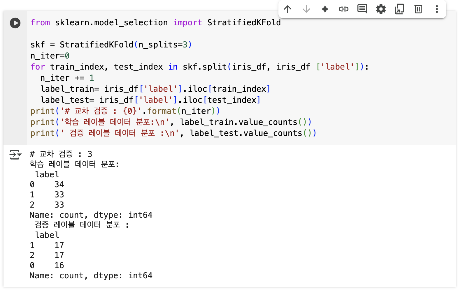

• 출력 결과를 보면 학습 레이블과 검증 레이블 데이터 값의 분포도가 거의 동일하게 할당됨.

• 전체 150 개의 데이터에서 학습으로 100 개, 검증으로 50 개가 교차 검증 단계별로 할당이 되었습니다.

• 첫 번째 교차 검증에서 100 개의 학습 레이블은 0, 1, 2 값이 각각 34, 33, 33 개로, 레이블 값별로 거의 동일하게 할당됐고,

• 50 개의 검증 레이블 역시 0, 1, 2 값이 각각 17, 17, 16 개로, 레이블 값별로 거의 동일하게 할당되었습니다.

• 이렇게 분할이 되어야 레이블 값 0, 1, 2 를 모두 학습할 수 있고, 이에 기반해 검증을 수행할 수 있습니다.

• StratifiedKFold 를 이용해 붓꽃 데이터를 교차 검증해 보겠습니다.

• 다음 코드는 StratifiedKFold 를 이용해 데이터를 분리한 것입니다.

• 피처 데이터와 레이블 데이터는 앞의 붓꽃 StratifiedKFold 예제에서 추출한 데이터를 그대로 이용하겠습니다.

from sklearn.tree import DecisionTreeClassifier
from sklearn.metrics import accuracy_score
from sklearn.model_selection import StratifiedKFold
from sklearn.datasets import load_iris
import numpy as np

# 데이터 로딩
iris = load_iris()
features = iris.data
label = iris.target

# 모델 및 StratifiedKFold 설정
dt_clf = DecisionTreeClassifier(random_state=156)
skfold = StratifiedKFold(n_splits=3)
n_iter = 0
cv_accuracy = []

# StratifiedKFold의 split() 호출 시 반드시 레이블 데이터 세트도 추가 입력 필요
for train_index, test_index in skfold.split(features, label):
    # split()으로 반환된 인덱스를 이용해 학습용, 검증용 테스트 데이터 추출
    X_train, X_test = features[train_index], features[test_index]
    y_train, y_test = label[train_index], label[test_index]

    # 학습 및 예측
    dt_clf.fit(X_train, y_train)
    pred = dt_clf.predict(X_test)

    # 반복 시마다 정확도 측정
    n_iter += 1
    accuracy = np.round(accuracy_score(y_test, pred), 4)
    train_size = X_train.shape[0]
    test_size = X_test.shape[0]

    print('\n#{0} 교차 검증 정확도 : {1}, 학습 데이터 크기 : {2}, 검증 데이터 크기 : {3}'
          .format(n_iter, accuracy, train_size, test_size))
    print('#{0} 검증 세트 인덱스 : {1}'.format(n_iter, test_index))

    cv_accuracy.append(accuracy)

# 교차 검증별 정확도 및 평균 정확도 계산
print('\n## 교차 검증별 정확도:', np.round(cv_accuracy, 4))
print('## 평균 검증 정확도:', np.round(np.mean(cv_accuracy), 4))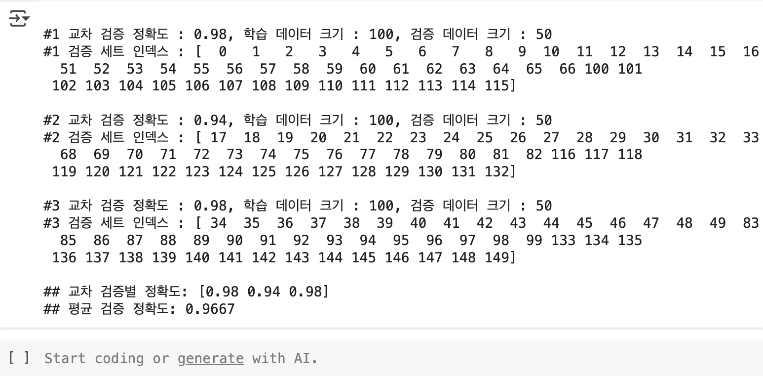

``

• 3 개의 Stratified K 폴드로 교차 검증한 결과 평균 검증 정확도가 약 96.67% 로 측정.

• Stratified K 폴드의 경우 원본 데이터의 레이블 분포도 특성을 반영한 학습 및 검증 데이터 세트를 만들 수 있으므로 왜곡된 레이블 데이터 세트에서는 반드시 Stratified K 폴드를 이용해 교차 검증해야 함.

• 분류(Classification) → Stratified K 폴드 자동 적용

• 회귀(Regression) → 기본 K 폴드 사용

• 회귀 (Regression) 에서는 Stratified K 폴드가 지원되지 않음.

• 회귀의 결정값은 이산값 형태의 레이블이 아니라 연속된 숫자값이기 때문에 결정값별로 분포를 정하는 의미가 없음.

교차 검증을 보다 간편하게 - cross_val_score()

• 사이킷런은 교차 검증을 좀 더 편리하게 수행할 수 있게 해주는 cross_val_score() 와 같은 API 를 제공합니다.

KFold 로 데이터를 학습하고 예측하는 코드를 보면
먼저
1. 폴드 세트를 설정
2. for 루프에서 반복으로 학습 및 테스트 데이터의 인덱스를 추출
3. 반복적으로 학습과 예측을 수행하고 예측 성능을 반환.

cross_val_score()는 이런 일련의 과정을 한꺼번에 수행해주는 API 입니다.

주요 파라미터 : estimator, X, y, scoring, cv

• estimator :
  사이킷런의 분류 알고리즘 클래스인 Classifier 또는 회귀 알고리즘 클래스인 Regressor
• X : 피처 데이터 세트, y 는 레이블 데이터 세트
• scoring : 예측 성능 평가 지표를 기술함
• cv : 교차 검증 폴드 수
  - cross_val_score() 수행 후 반환 값은 scoring 파라미터로 지정된 성능 지표 측정값을 배열 형태로 반환.
• cross_val_score()는 classifier가 입력되면 Stratified K 폴드 방식으로 레이블값의 분포에 따라 학습/테스트 세트를 분할함

회귀인 경우는 Stratified K 폴드 방식으로 분할할 수 없으므로 K 폴드 방식으로 분할합니다

• 아래 코드는 교차 검증 폴드 수는 3, 성능 평가 지표는 정확도인 accuracy

from sklearn.tree import DecisionTreeClassifier
from sklearn.model_selection import cross_val_score, cross_validate
from sklearn.datasets import load_iris
iris_data = load_iris()
dt_clf = DecisionTreeClassifier(random_state=156)
data = iris_data.data
label = iris_data. target
# 성능 지표는 정확도 (accuracy), 교차 검증 세트는 3 개
scores = cross_val_score(dt_clf, data, label, scoring='accuracy', cv=3)
print('교차 검증별 정확도 :' , np.round(scores, 4))
print('평균 검증 정확도 :', np.round(np.mean(scores), 4))

실행 결과는 이렇게 나옴

교차 검증별 정확도 : [0.98 0.94 0.98]
평균 검증 정확도 : 0.9667

• cross_val_score()는 cv로 지정된 횟수만큼 scoring 파라미터로 지정된 평가 지표로 평가 결과 값을 배열로 반환.

• 일반적으로 이를 평균해 평가 수치로 사용합니다.

• cross_val_score() API는 내부에서 Estimator를 학습 (fit), 예측 (predict), 평가 (evaluation) 시켜주므로 간단하게 교차 검증을 수행 가능.

• 붓꽃 데이터의 cross_val_score() 수행 결과와 앞 예제의 붓꽃 데이터 StratifiedKFold의 수행 결과를 비교해 보면 각 교차 검증별 정확도와 평균 검증 정확도가 모두 동일함. (cross_val_score()가 내부적으로 StratifiedKFold를 이용하기 때문임)

• 비슷한 API로 cross_validate()있음.

• cross_val_score() : 단 하나의 평가 지표만 가능

• cross_validate() : 여러 개의 평가 지표를 반환 가능

GridSearchCV - 교차 검증과 최적 하이퍼 파라미터 튜닝을 한 번에

• 하이퍼 파라미터는 알고리즘의 성능에 중요한 영향을 주는 요소

• GridSearchCV는 하이퍼 파라미터 튜닝을 자동화하는 사이킷런의 주요 도구

• Grid 방식은 가능한 조합을 촘촘하게 테스트해 최적값 탐색

• 아직 상세 설명 전이지만, 튜닝 방식에 대한 사전 이해가 중요

• 사이킷런은 GridSearchCV API 를 이용해 Classifier나 Regressor와 같은 알고리즘에 사용되는 하이퍼 파라미터를 순차적으로 입력하면서 편리하게 최적의 파라미터를 도출할 수 있는 방안을 제공

Grid 는 격자라는 뜻으로, 촘촘하게 파라미터를 입력하면서 테스트를 하는 방식입니다

• 예) 결정 트리 알고리즘의 여러 하이퍼 파라미터를 순차적으로 변경하면서 최고 성능을 가지는 파라미터 조합을 찾기

grid_parameters = {'max_depth': [1, 2, 3],
                    'min_samples_split': [2, 3]}

• 하이퍼 파라미터는 다음과 같이 순차적으로 적용되며, 총 6 회에 걸쳐 파라미터를 순차적으로 바꿔 실행하면서 최적의 파라미터와 수행 결과를 도출할 수 있음
• GridSearchCV 는 교차 검증을 기반으로 이 하이퍼 파라미터의 최적 값을 찾게 해줌.
• 사용자가 튜닝하고자 하는 여러 종류의 하이퍼 파라미터를 다양하게 테스트하면서 최적의 파라미터를 편리하게 찾게 해주지만
  동시에 순차적으로 파라미터를 테스트하므로 수행시간이 상대적으로 오래 걸리는 것에 유념해야 함.
• CV가 3회라면 개별 파라미터 조합마다 3개의 폴딩 세트를 3 회에 걸쳐 학습/평가해 평균값으로 성능을 측정함
• 6개의 파라미터 조합이라면 총 CV 3회 X 6개 파라미터 조합 = 18 회의 학습/평가가 이뤄짐.

GridSearchCV 클래스의 생성자로 들어가는 주요 파라미터

• estimator : classifier, regressor, pipeline 이 사용될 수 있음.
• param_grid : key + 리스트 값을 가지는 딕셔너리가 주어집니다. estimator의 튜닝을 위해 파라미터명과 사용될 여러 파라미터 값을 지정.
• scoring: 예측 성능을 측정할 평가 방법을 지정합니다. 보통은 사이킷런의 성능 평가 지표를 지정하는 문자열 ( 예 : 정확도의 경우 'accuracy')로 지정하나 별도의 성능 평가 지표 함수도 지정할 수 있습니다.
• cv: 교차 검증을 위해 분할되는 학습 / 테스트 세트의 개수를 지정합니다.
• refit: 디폴트가 True 이며 True 로 생성 시 가장 최적의 하이퍼 파라미터를 찾은 뒤 입력된 estimator 객체를 해당 하이퍼 파라미터로 재학습시킴.

• 결정 트리 알고리즘의 여러 가지 최적화 파라미터를 순차적으로 적용해 붓꽃 데이터를 예측 분석하는 데 GridSearchCV를 이용
• train_test_split() 을 이용해 학습 데이터와 테스트 데이터를 먼저 분리하고 학습 데이터에서 GridSearchCV 를 이용해 최적 하이퍼 파라미터를 추출.
• 결정 트리 알고리즘을 구현한 DecisionTreeClassifier 의 중요 하이퍼 파라미터인 max_depth 와 min_samples_split 의 값을 변화시키면서 최적화를 진행
• 테스트할 하이퍼 파라미터 세트는 딕셔너리 형태로
  하이퍼 파라미터의 명칭은 문자열 Key 값으로, 하이퍼 파라미터의 값은 리스트 형으로 설정.

from sklearn.datasets import load_iris
from sklearn.tree import DecisionTreeClassifier
from sklearn.model_selection import GridSearchCV
from sklearn.model_selection import train_test_split
# 데이터를 로딩하고 학습 데이터와 테스트 데이터 분리
iris_data = load_iris()
X_train, X_test, y_train, y_test = train_test_split(iris_data.data, iris_data.target,
                                                    test_size=0.2, random_state=121)
dtree = DecisionTreeClassifier()
### 파라미터를 딕셔너리 형태로 설정
parameters = {'max_depth':[1, 2, 3], 'min_samples_split': [2, 3]}

• 학습 데이터 세트를 GridSearchCV 객체의 fit(학습 데이터 세트) 메서드에 인자로 입력
  - fit() 수행 시, cv 폴딩 세트로 분할 → param_grid의 하이퍼 파라미터 순차 변경 → 학습/평가
• 결과는 cvresults 속성에 기록 (딕셔너리 형태)
• cvresults를 Pandas DataFrame으로 변환하면 내용 확인 쉬움
• 주요 칼럼으로 GridSearchCV 동작 방식 파악 가능

import pandas as pd
# paran_grid 의 하이퍼 파라미터를 3 개의 train, test set fold 로 나누어 테스트 수행 설정.
## refit=True가 default임. True 이면 가장 좋은 파라미터 설정으로 재학습시킴.
grid_dtree = GridSearchCV(dtree, param_grid=parameters, cv=3, refit=True)
# 붓꽃 학습 데이터로 param grid의 하이퍼 파라미터를 순차적으로 학습 / 평가 .
grid_dtree. fit(X_train, y_train)
#GridsearchcV 결과를 추출해 Dataframe 으로 변환
scores_df = pd.DataFrame(grid_dtree.cv_results_)
scores_df[['params', 'mean_test_score', 'rank_test_score',
           'split0_test_score', 'split1_test_score', 'split2_test_score']]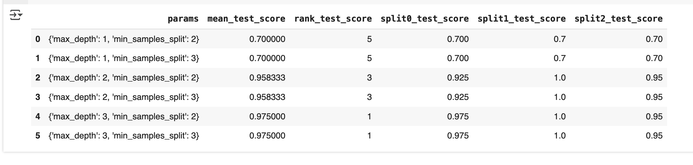

• 총 6 개의 결과는 하이퍼 파라미터 max_depth와 min_samples_split을 6 번 변경하며 학습/평가한 것
• params 칼럼: 적용된 하이퍼 파라미터 값
• 인덱스 4, 5번 행의 rank_test_score 값이 1 → 공동 1위 성능
• 해당 mean_test_score 값: 0.975000 (가장 높음)
• split0_test_score, split1_test_score, split2_test_score: CV=3에서 각 폴드의 성능
• mean_test_score: 위 세 값의 평균

주요 칼럼별 의미

• params 칼럼 : 수행할 때마다 적용된 개별 하이퍼 파라미터값

• rank_test_score: 하이퍼 파라미터별 성능 순위 (1이 최적의 하이퍼 파라미터)

• mean_test_score : 하이퍼 파라미터별로 CV 폴딩 테스트 세트에 대한 평균 평가값

• GridSearchCV 객체의 fit() 을 수행하면 최고 성능을 나타낸 하이퍼 파라미터 값과 평가 결과 값이 각각 bestparams, bestscore 속성에 기록됨
  cv_results의 ranktest_score가 1일 때의 값

• 이 속성을 이용해 최적 하이퍼 파라미터와 정확도를 확인할 수 있음

print('Gridsearchcv 최적 파라미터 :', grid_dtree.best_params_)
# GridsearchcV 최적 파라미터 : ('max_depth': 3 , 'min_samples_split : 2} 출력
print('GridsearchCV 최고 정확도:{0:.4f}'.format(grid_dtree.best_score_))
# GridSearchcV 최고 정확도 : 0.9750 출력

• max_depth가 3, min_samples_split이 2일 때 평균 최고 정확도는 97.50%

• GridSearchCV는 기본 파라미터 refit=True

• refit=True이면 최적 하이퍼파라미터로 Estimator 재학습 후 bestestimator로 저장

• bestestimator를 사용해 train_test_split()으로 나눈 테스트 세트에 예측 및 성능 평가 가능

# GridSearchcV의 refit으로 이미 학습된 estimator 반환
estimator = grid_dtree.best_estimator_
# Gridsearchcv의 best_estimator_는 이미 최적 학습이 됐으므로 별도 학습이 필요 없음
pred = estimator.predict(X_test)
print('테스트 데이터 세트 정확도 : {0: 4f}'.format(accuracy_score(y_test, pred)))

#  출력 |||| 테스트 데이터 세트 정확도 :  0.966667

• 테스트 세트 정확도: 96.67% 를 의미
• GridSearchCV로 튜닝 후 별도 테스트 세트로 평가하는 것이 일반적 방법

5. 데이터 전처리 (Data Preprocessing)

• ML 알고리즘만큼 중요
• 사이킷런의 ML 알고리즘은 NaN, Null 값 허용하지 않음
• Null 값은 평균값 등으로 대체하거나, 대부분일 경우 피처 삭제 고려
• Null 값이 일정 수준 이상일 경우 → 더 정밀한 대체 값 필요
• 사이킷런 알고리즘은 문자열 입력 허용 안 함 → 숫자형으로 인코딩 필요
• 카테고리형 피처는 코드 값으로 표현
• 텍스트형 피처는 벡터화 또는 삭제
• 주민번호, 아이디 등 식별자 피처는 삭제가 바람직 (예측 성능 저하 유발)
• 텍스트형 피처 → 피처 벡터화 (feature vectorization) 필요

데이터 인코딩

• 대표적인 인코딩 방식: 레이블 인코딩과 원-핫 인코딩 (One Hot encoding)
• 레이블 인코딩은 카테고리 피처를 코드형 숫자 값으로 변환
• 예: TV → 1, 냉장고 → 2, 전자레인지 → 3, 컴퓨터 → 4, 선풍기 → 5, 믹서 → 6
• 주의: '01', '02' 같은 문자열 코드도 숫자형으로 변환 필요

레아블 인코딩 (Label encoding)

• LabelEncoder 클래스로 구현
• LabelEncoder 를 객체로 생성한 후 fit() 과 transform()을 호출해 레이블 인코딩을 수행

from sklearn.preprocessing import LabelEncoder
items=['TV', '냉장고' , '전자레인지' , '컴퓨터', '선풍기'  , '선풍기' , '믹서', '믹서']
# LabelEncoder를 객체로 생성한 후 , fit() 과 transform() 으로 레이블 인코딩 수행.
encoder = LabelEncoder()
encoder.fit(items)
labels = encoder.transform(items)
print('인코딩 변환값:', labels)

# 출력 |||| 인코딩 변환값: [0 1 4 5 3 3 2 2]

• TV 는 0, 냉장고는 1, 전자레인지는 4, 컴퓨터는 5, 선풍기는 3, 믹서는 2 로 변환됨
• 데이터가 작으면 인코딩 결과를 직관적으로 확인 가능
• 데이터가 많을 경우 LabelEncoder 객체의 classes_ 속성으로 확인 가능

print('인코딩 클래스 :' , encoder.classes_)
# 출력 ||| 인코딩 클래스 : [' 선풍기 , 선풍기 , 믹서, 믹서 ' ' 컴퓨터 ' 'TV' '냉장고' '전자레인지']

원- 핫 인코딩 (One-Hot Encoding)

• 원-핫 인코딩은 고유 값마다 새로운 피처를 추가하고, 해당 칼럼에만 1, 나머지는 0을 표시
• 행 형태의 피처 고유 값을 열 형태로 변환
• 고유 값이 6개이면 → 6개의 새로운 피처로 변환
• 예: 상품 분류가 TV면 '상품_분류_TV'에만 1, 나머지는 0
• 이런 방식 때문에 ‘원-핫(One-Hot)’ 인코딩이라 부름
• 사이킷런에서는 OneHotEncoder 클래스로 변환 가능
• 주의사항: 입력은 2차원 데이터여야 함
• 반환값은 희소 행렬(Sparse Matrix) → .toarray()로 밀집 행렬(Dense Matrix)로 변환해야

from sklearn.preprocessing import OneHotEncoder
import numpy as np
items= ['TV', '냉장고','전자레인지', '컴퓨터' ,'선풍기' , '선풍기' , '믹서' , '믹서' ]
# 2차원 ndarray로 변환합니다.
items = np.array(items).reshape(-1, 1)
# 원- 핫 인코딩을 적용합니다.
oh_encoder = OneHotEncoder()
oh_encoder. fit(items)
oh_labels = oh_encoder.transform(items)
# OnetotEncoder로 변환한 결과는 희소행렬이므로 toarray()를 이용해 밀집 행렬로 변환.
print('원-핫 인코딩 데이터')
print(oh_labels. toarray())
print('원-핫 인코딩 데이터 차원 ')
print(oh_labels.shape)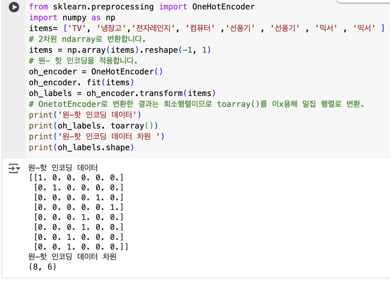

• 8 개의 레코드와 1 개의 칼럼 → 8 개의 레코드와 6 개의 칼럼으로 변환
• TV: 0, 냉장고: 1, 믹서: 2, 선풍기: 3, 전자레인지: 4, 컴퓨터: 5
• 첫 번째 칼럼: TV, 두 번째 칼럼: 냉장고, ... 여섯 번째 칼럼: 컴퓨터
• 원본 첫 번째 레코드가 TV → 변환된 첫 번째 레코드의 첫 번째 칼럼 = 1, 나머지 = 0
• 두 번째 레코드가 냉장고 → 변환된 두 번째 레코드의 두 번째 칼럼 = 1, 나머지 = 0
• get_dummies() 를 이용하면 됨 --- 사이킷런의 OneHotEncoder와 다르게 문자열 카테고리 값을 숫자 형으로 변환할 필요 없이 바로 변환 가능

import pandas as pd
df= pd.DataFrame({'item':['TV', '냉장고' ,'전자레인지' ,'컴퓨터' , '선풍기' , '선풍기' , '믹서' , '믹서']
})
pd.get_dummies(df)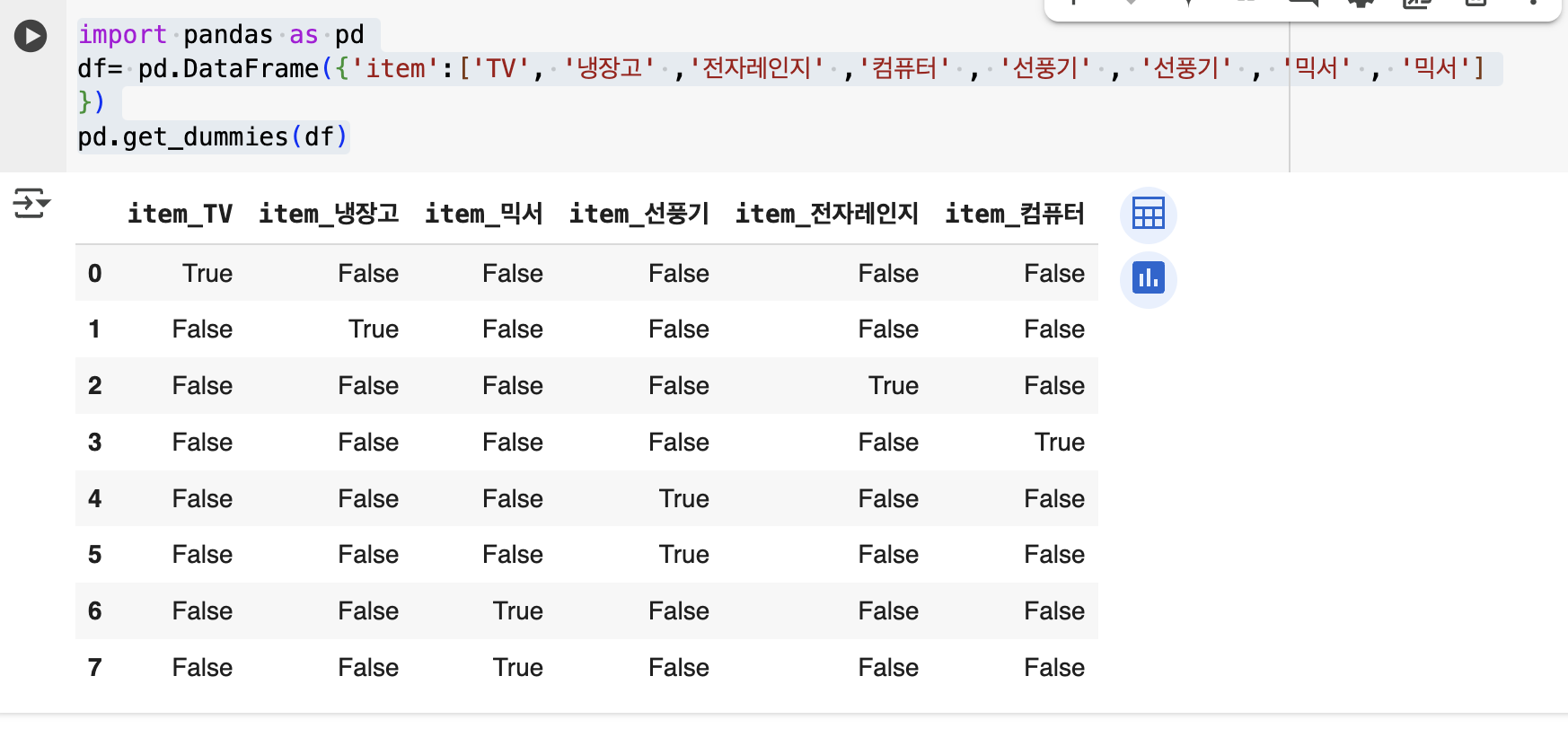

피처 스케일링과 정규화

• 서로 다른 변수의 값 범위를 일정한 수준으로 맞추는 작업을 피처 스케일링 (feature scaling)이라고 함

- 대표적인 방법
1. 표준화 (Standardization)
2. 정규화 (Normalization)

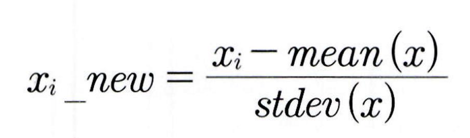
• 표준화는 평균이 0, 분산이 1인 가우시안 정규 분포로 변환
• 변환된 값은 원래 값에서 피처의 평균을 빼고, 표준편차로 나눈 값으로 계산됨
  

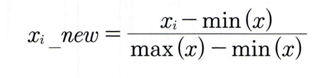
일반적으로 정규화는 서로 다른 피처의 크기를 통일하기 위해 크기를 변환하는 개념

예:
피처 A: 거리 (0 ~ 100KM)
피처 B: 금액 (0 ~ 100,000,000원)
모든 값을 0 ~ 1 사이로 변환해 동일 단위로 비교

새로운 데이터는 원래 값에서 피처의 최솟값을 빼고, 최댓값과 최솟값의 차이로 나눈 값으로 변환됨

• 사이킷런의 전처리에서 제공하는 Normalizer 모듈과 일반적인 정규화는 약간 차이 있음
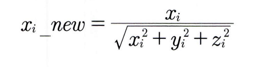
• 큰 개념은 같지만, 사이킷런 Normalizer는 선형대수의 정규 개념 적용
• 개별 벡터의 크기를 맞추기 위해 변환
• 개별 벡터를 모든 피처 벡터의 크기로 나눠 줌

혼선을 방지하기 위해

• 일반적인 표준화와 정규화 → 피처 스케일링
• 선형대수 개념의 정규화 → 벡터 정규화로 지칭

사이킷런의 대표적인 피처 스케일링 클래스

• StandardScaler
• MinMaxScaler

StandardScaler

• StandardScaler는 표준화를 지원하는 클래스임
• 개별 피처를 평균 0, 분산 1인 값으로 변환
• 가우시안 정규 분포를 가지도록 변환
• 표준화는 예측 성능 향상에 중요한 요소

특히 중요한 알고리즘:

• SVM (RBF 커널)
• 선형 회귀 (Linear Regression)
• 로지스틱 회귀 (Logistic Regression)

from sklearn.datasets import load_iris
import pandas as pd
# 붓꽃 데이터 세트를 로딩하고 Dataframe 으로 변환합니다.
iris = load_iris()
iris_data = iris.data
iris_df = pd.DataFrame(data=iris_data, columns=iris.feature_names)
print('feature 들의 평균 값 ')
print(iris_df.mean())
print('Infeature 들의 분산 값 ')
print(iris_df.var())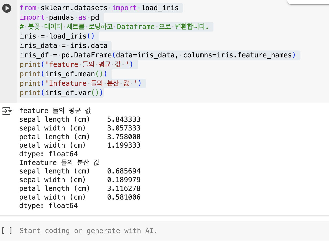

• StandardScaler를 이용해 각 피처를 한 번에 표준화
• StandardScaler 객체 생성 후
• fit()과 transform() 메서드에 변환 대상 피처 데이터 세트 입력하여 호출

from sklearn.preprocessing import StandardScaler
# StandardScaler 객체 생성
scaler = StandardScaler()
# StandardScaler로 데이터 세트 변환. fit()과 transform( ) 호출.
scaler.fit(iris_df)
iris_scaled = scaler.transform(iris_df)
# transform() 시 스케일 변환된 데이터 세트가 NumPy ndarray로 반환돼 이를 Dataframe 으로 변환
iris_df_scaled = pd.DataFrame(data=iris_scaled, columns=iris.feature_names)
print('feature 들의 평균 값 ' )
print(iris_df_scaled.mean())
print('Infeature 들의 분산 값')
print(iris_df_scaled.var())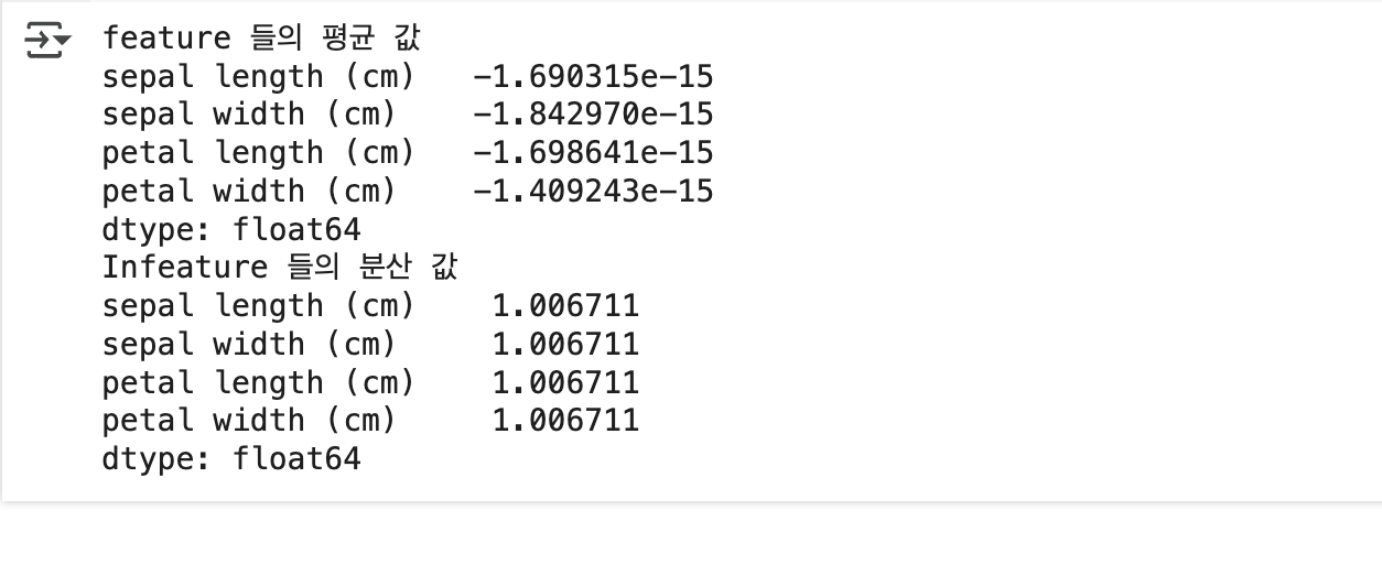

모든 칼럼 값의 평균이 0 에 아주 가까운 값으로 ,
그리고 분산은 1 에 아주 가까운 값으로 변환됨

MinMaxScaler

• MinMaxScaler는 데이터값을 0과 1 사이로 변환
• 음수 값이 있으면 -1에서 1 사이로 변환
• 데이터 분포가 가우시안 분포가 아닐 경우 → Min, Max Scale 적용 고려 가능

from sklearn.preprocessing import MinMaxScaler
# MinMaxScaler 객체 생성
scaler = MinMaxScaler()
# MinMaxScaler 로 데이터 세트 변환. fit()과 transform() 호출.
scaler.fit(iris_df)
iris_scaled = scaler.transform(iris_df)
# transform() 시 스케일 변환된 데이터 세트가 NumPy ndarray로 반환돼 이를 Dataframe으로 변환
iris_f_scaled = pd.DataFrame(data=iris_scaled, columns=iris.feature_names)
print('feature들의 최솟값')
print(iris_df_scaled.min())
print('Infeature들의 최댓값')
print(iris_df_scaled.max())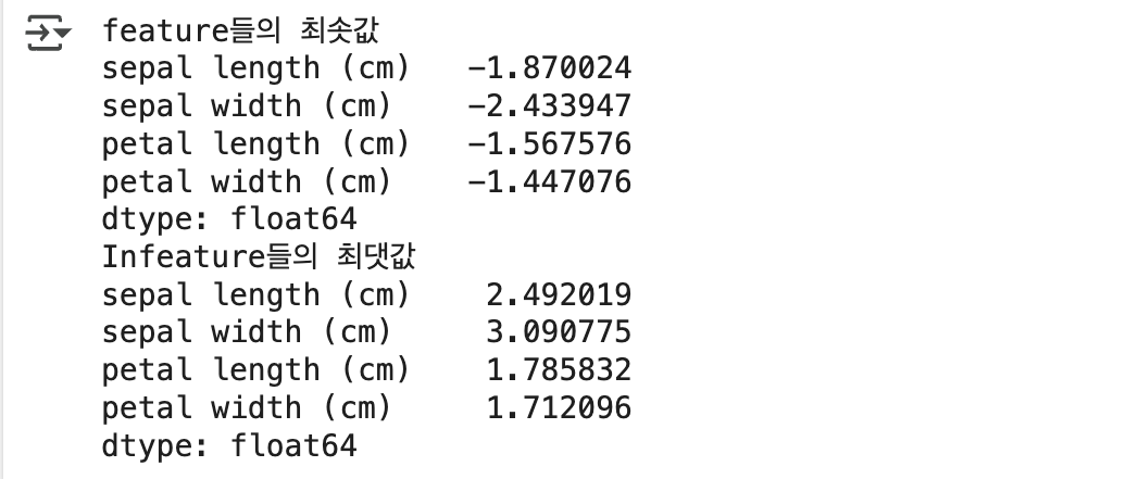

학습 데이터와 테스트 데이터의 스케일링 변환 시 유의점

• StandardScaler, MinMaxScaler 사용 시 fit(), transform(), fit_transform() 메서드 이용
• fit()은 변환 기준 정보 설정, transform()은 설정된 기준으로 변환
• fit_transform()은 두 과정을 한 번에 수행

주의점:

• 학습 데이터에 fit()과 transform() 적용 후
• 테스트 데이터에는 fit() 없이 transform()만 적용해야 함
• 테스트 데이터에 다시 fit()하면 학습/테스트의 스케일 기준이 달라져 잘못된 예측 가능성

from sklearn.preprocessing import MinMaxScaler
import numpy as np
# 학습 데이터는 0 부터 10 까지 , 테스트 데이터는 0 부터 5 까지 값을 가지는 데이터 세트로 생성
# Scaler 클래스의 fit(), transform() 은 2 차원 이상 데이터만 가능하므로 reshape(-1, 1) 로 차원 변경
train_array = np.arange(0, 11) .reshape(-1, 1)
test_array = np.arange(0, 6). reshape(-1, 1)

학습 데이터 train_array에 MinMaxScaler 적용
데이터: 0부터 10까지 값
fit() 적용 시 → 최솟값 0, 최댓값 10 설정 → 1/10 스케일 적용

• transform() 호출 시 →
  1 → 0.1
  2 → 0.2
  5 → 0.5
  10 → 1

# MinMaxScaler 객체에 별도의 feature_range 파라미터 값을 지정하지 않으면 0~1 값으로 변환
scaler = MinMaxScaler()
# fit()하게 되면 train_array 데이터의 최솟값이 0, 최댓값이 10 으로 설정.
scaler.fit(train_array)
# 1/10 scale 로 train_array 데이터 변환함. 원본 10- 〉 1 로 변환됨.
train_scaled = scaler. transform(train_array)
print('원본 train_array 데이터 :', np.round (train_array.reshape(-1), 2))
print('Scale된 train_array 데이터:', np.round(train_scaled.reshape(-1), 2))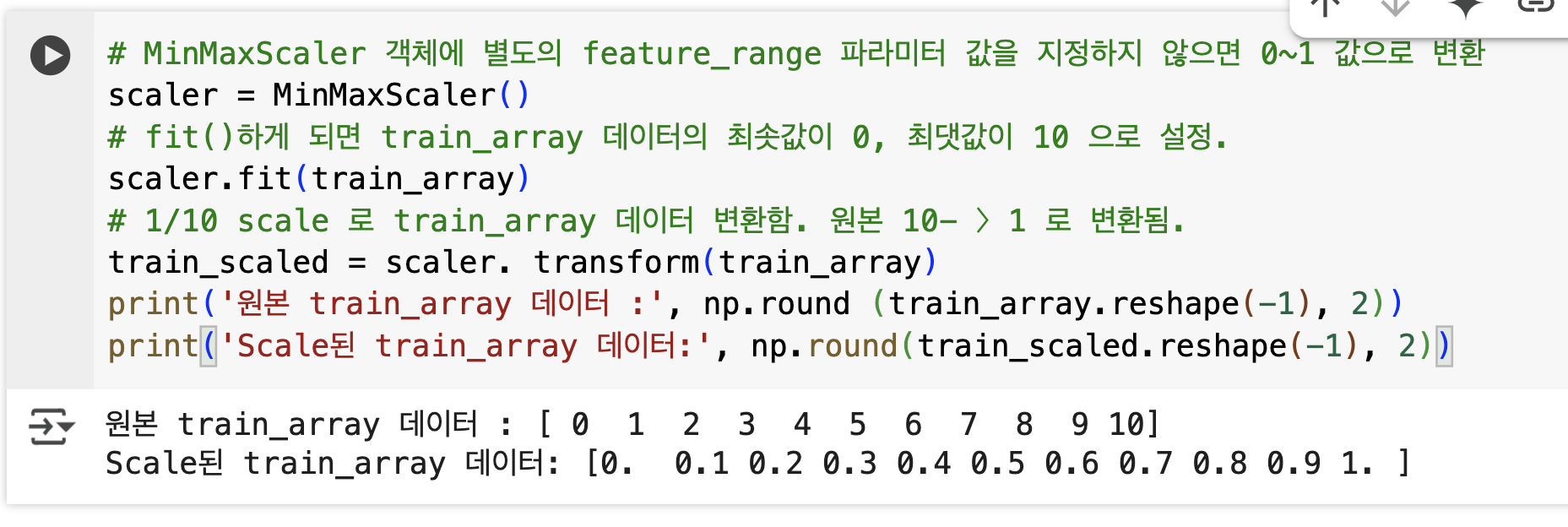

# MinMaxScaler 에 test_array를 fit()하게 되면 원본 데이터의 최솟값이 0, 최댓값이 scaler. fit(test_array)
#5 로 설정됨
# 1/5 scale로 test_array 데이터 변함. 원본 5->1로 변환.
test_scaled = scaler. transform(test_array)
# test_array의 Scale 변환 출력.
print('원본 test_array 데이터 :', np.round(test_array.reshape(-1), 2))
print('Scale된 test_array 데이터:', np.round(test_scaled.reshape(-1), 2))

윗부분 코드가 출력이 이렇게 됩니다.

원본 test_array 데이터 : [0 1 2 3 4 5]
Scale된 test_array 데이터: [0.  0.1 0.2 0.3 0.4 0.5]

• 출력 결과: 학습 데이터와 테스트 데이터의 스케일링이 맞지 않음

• 테스트 데이터는 최솟값 0, 최댓값 5 → 1/5 스케일
  1 → 0.2, 5 → 1

• 학습 데이터는 1/10 스케일
  2 → 0.2, 10 → 1

• 서로 다른 원본값이 같은 값으로 변환됨 → 잘못된 결과

• 테스트 데이터는 학습 데이터의 스케일링 기준을 따라야 함

• 테스트 데이터는 다시 fit() 하면 안 됨, 학습 데이터로 fit()된 Scaler로 transform()만 적용

• 결과: 학습/테스트 데이터 모두 1/10 수준으로 동일하게 스케일링

scaler = MinMaxScaler()
scaler.fit(train_array)
train_scaled = scaler. transform(train_array)
print('원본 train_array 데이터 :', np.round(train_array.reshape(-1), 2))
print('Scale train_array 데이터:', np.round(train_scaled.reshape(-1), 2))
# test_array에 Scale 변환을 할 때는 반드시 fit()을 호출하지 않고 transform()만으로 변환해야 함.
test_scaled = scaler.transform(test_array)
print('\n원본 test_array 데이터 :' , np.round(test_array.reshape(-1), 2))
print('Scale된 test_array 데이터 :', np.round(test_scaled.reshape(-1), 2))

• fit_transform()은 fit()과 transform()을 순차적으로 수행
• 학습 데이터에는 사용 가능, 테스트 데이터에서는 절대 사용 금지
• 학습과 테스트에 fit()과 transform() 적용 시 주의 사항 발생
• 따라서 스케일링은 전체 데이터에 먼저 적용 후, 학습/테스트 세트로 분리하는 것이 바람직

학습 데이터와 테스트 데이터의 fit(), transform(), fit_transtorm()을 이용해 스케일링 변환 시 유의할 점

1. 가능하다면 전체 데이터의 스케일링 변환을 적용한 뒤 학습과 테스트 데이터로 분리
2. 1 이 여의치 않다면 테스트 데이터 변환 시에는 fit( ) 이나 fit_transform() 을 적용하지 않고 학습 데이터로 이미 fit()
   된 Scaler 객체를 이용해 transform( ) 으로 변환

---

6. 사이킷런으로 수행하는 타이타닉 생존자 예측

https://colab.research.google.com/drive/1K5avPMjL-bXZLhmycFRVBhgx7hNwtKNJ?usp=sharing

• Passengerid: 탑승자 데이터 일련번호
• survived: 생존 여부 , 0= 사망 , 1= 생존
• pclass: 티켓의 선실 등급 , 1= 일등석 , 2= 이등석 , 3= 삼등석
• Sex: 탑승자 성별
• name: 탑승자 이름
• Age: 탑승자 나이
• Sibsp: 같이 탑승한 형제자매 또는 배우자 인원수
• parch: 같이 탑승한 부모님 또는 어린이 인원수
• ticket: 티켓 번호
• fare: 요금
• cabin: 선실 번호
• embarked: 중간 정착 항구 C=Cherbourg, Q=Queenstown, S= Southampton

1. 새로운 주피터 노트북을 생성
2. 분석에 필요한 라이브러리를 임포트한 후 타이타닉 탑승자 파일을 판다스의 read_csv()를 이용해 DataFrame 으로 로딩

import numpy as np
import pandas as pd
import matplotlib.pyplot as plt
import seaborn as sns
%matplotlib inline
titanic_df = pd.read_csv('sample_data/train.csv')
titanic_df.head(3)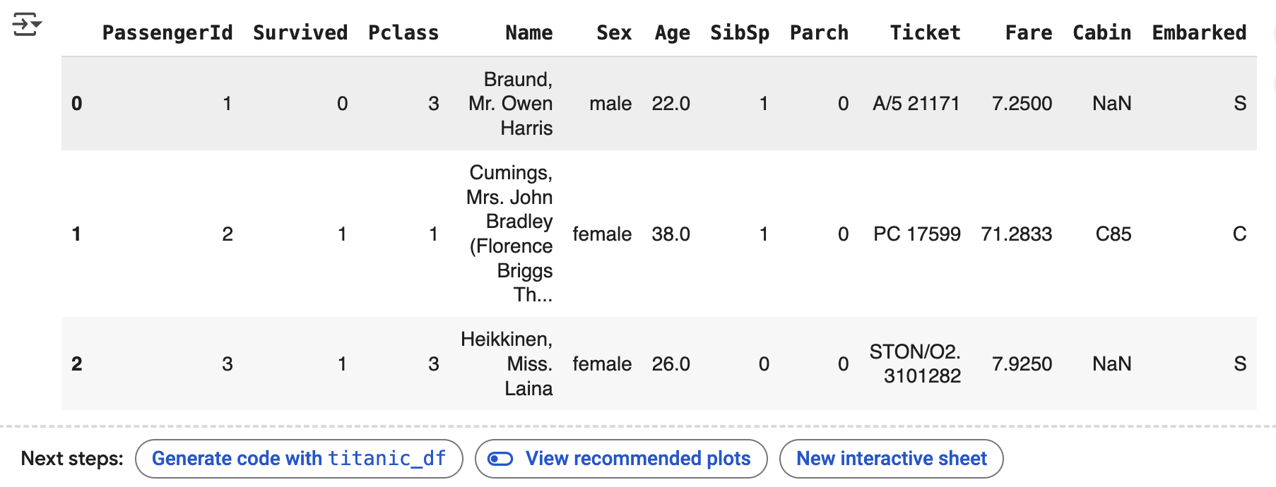

로딩된 데이터 컬럼 타입 확인

DataFrame 의 info() 메서드를 통해 쉽게 확인이 가능

print('\n ### 학습 데이터 정보 ### \n')
print(titanic_df.info())

• RangeIndex는 DataFrame 인덱스의 범위, → 891개 로우 (RangeIndex 가 891 entries)
• 총 12개 칼럼: float64: 2개, int64: 5개, object: 5개 → 문자열로 간주 가능
• Age, Cabin, Embarked 칼럼: 각각 177개, 608개, 2개 Null 값(NaN)
• 사이킷런 알고리즘은 Null 값 허용하지 않음

처리 방법:

• fillna() 함수 사용
• Age → 평균값으로
• 나머지 칼럼 → 'N'으로
• 이후 Null 값 제거 여부 확인 필수

titanic_df ['Age'].fillna(titanic_df['Age'].mean(), inplace=True)
titanic_df[ 'Cabin'].fillna('N', inplace=True)
titanic_df['Embarked'].fillna('N', inplace=True)
print('데이터 세트 Null 값 개수', titanic_df.isnull().sum().sum())

출력이 이렇게 나옵니다.

데이터 세트 Null 값 개수 0

print(' Sex 값 분포 :\n', titanic_df['Sex'].value_counts())
print('\n Cabin 값 분포 :\n', titanic_df ['Cabin'].value_counts())
print('\n Embarked 값 분포:\n', titanic_df ['Embarked' ].value_counts())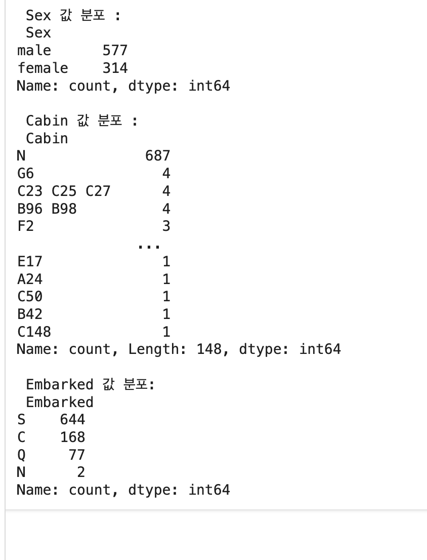

• Sex, Embarked 값은 별문제 없음
• Cabin은 'N'이 687건으로 가장 많고, 여러 Cabin이 한꺼번에 표기된 값도 있음 (C23 C25 C27 등 4건)
• Cabin은 속성값 정리가 제대로 안되어 있음
• 선실 등급을 나타내는 첫 번째 알파벳이 중요 → Cabin 속성은 앞 문자만 추출 예정

titanic_df['Cabin'] = titanic_df['Cabin'].str[:1]
print(titanic_df['Cabin'].head(3))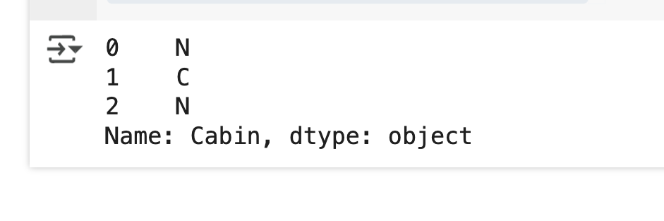

• 머신러닝 알고리즘 적용 전 데이터 탐색 수행
• 첫 번째 탐색: 어떤 유형의 승객이 생존 확률이 높았는지 확인
• 여성, 아이들, 노약자가 우선 구조 대상 (Women and Children First)
• 부자나 유명인도 구조 우선 대상
• 삼등실의 가난한 사람들은 생존률이 낮았을 가능성 → 성별에 따른 생존자 수 비교 예정

titanic_df.groupby(['Sex', 'Survived'])['Survived' ].count()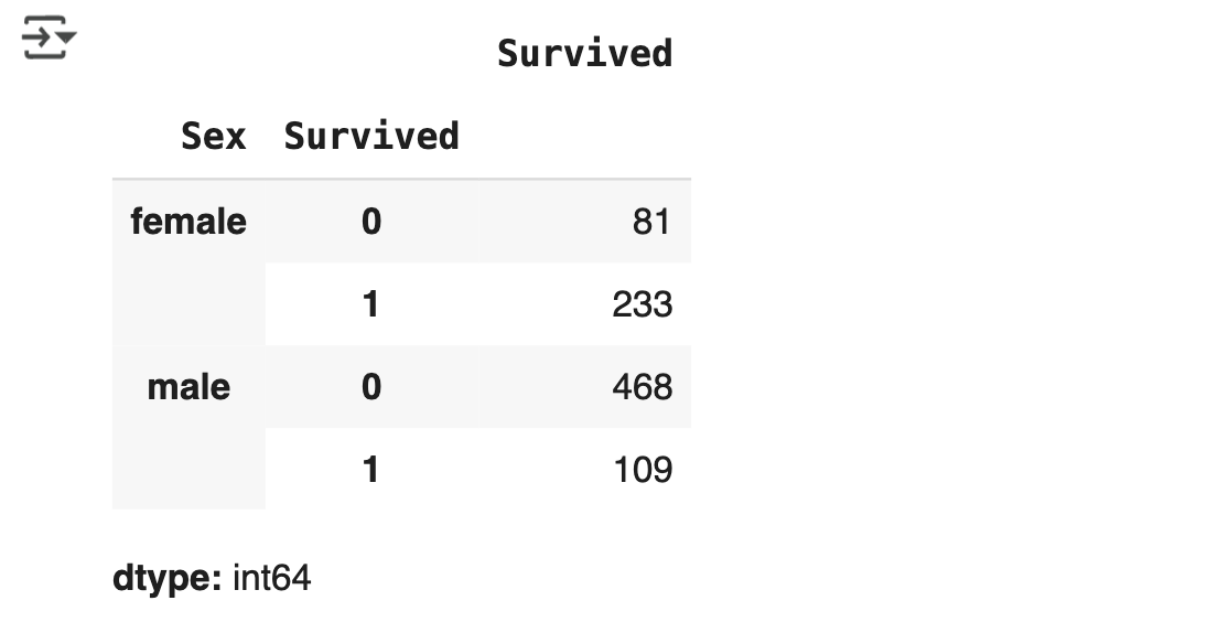

• Survived 칼럼은 레이블 (결정 클래스)

• 0: 사망, 1: 생존

• 탑승객 수: 남자 577명, 여자 314명

• 생존율:
  여자: 314명 중 233명 생존 → 약 74.2%
  남자: 577명 중 109명 생존 → 약 18.8%

• Seaborn 패키지로 시각화 진행
  X축: Sex, Y축: Survived

• barplot() 함수 사용

• DataFrame 객체 입력하여 막대 차트 출력

sns.barplot(x='Sex', y = 'Survived', data=titanic_df)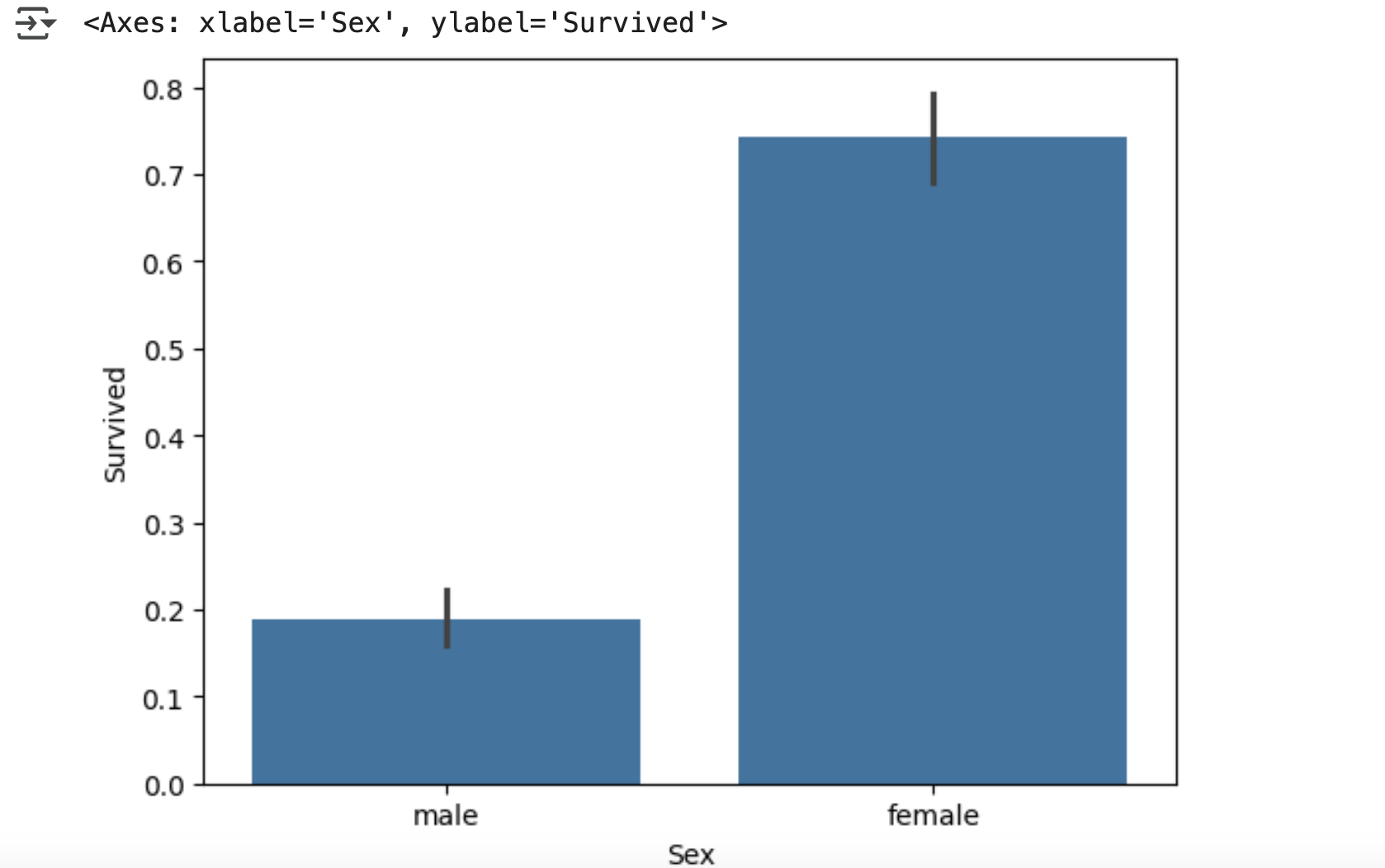

• 부자와 가난한 사람의 생존 확률 비교
• 객실 등급(Pclass)을 부의 기준으로 사용
• 일등실, 이등실, 삼등실에 따라 생존 확률 분석
• 성별도 함께 고려해 분석
• barplot() 함수에:
  x='Pclass', hue='Sex' 설정 → 객실 등급별 성별 생존 확률 시각화

sns.barplot(x='Pclass', y='Survived', hue='Sex', data=titanic_df)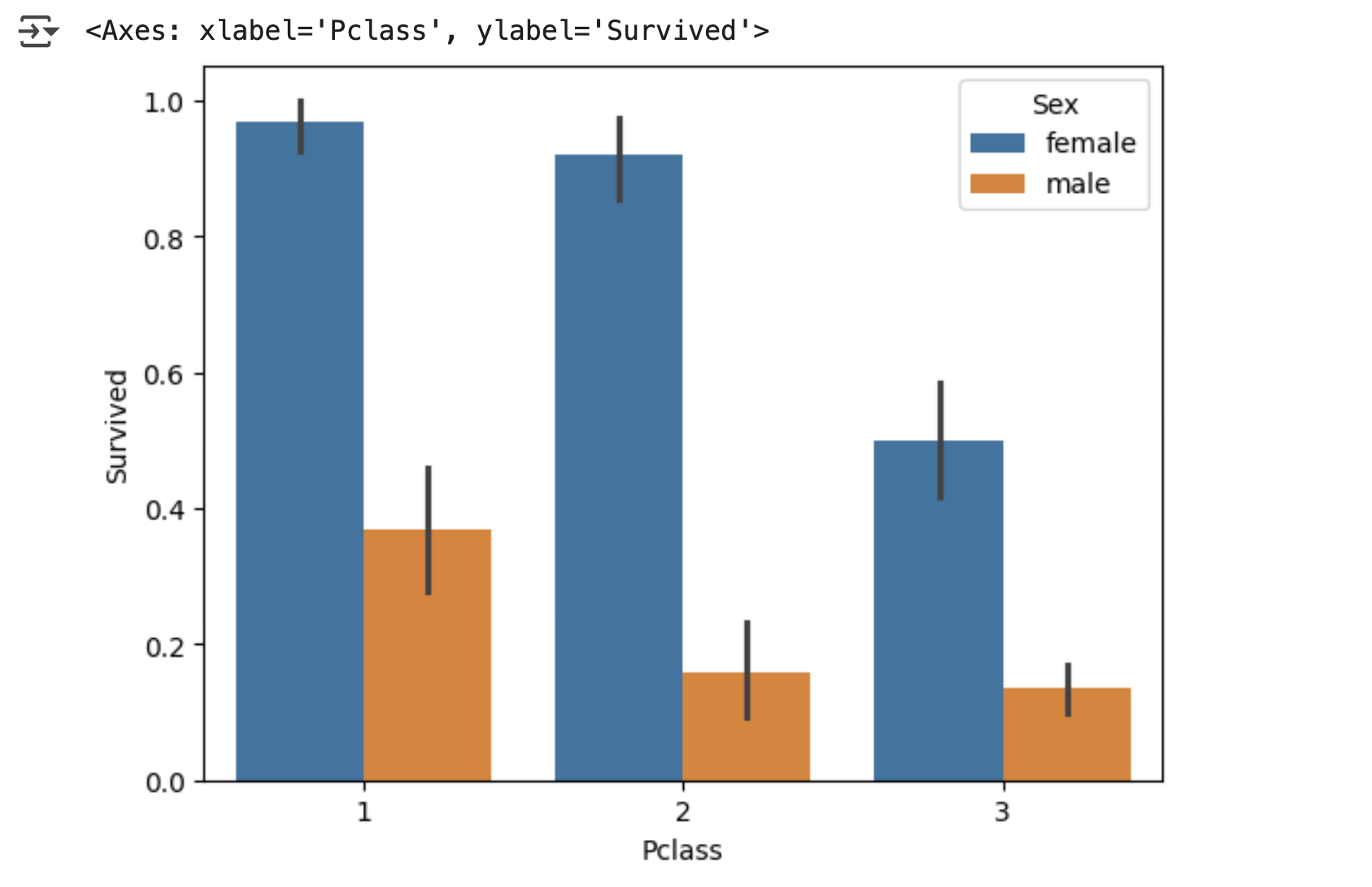

• 여성: 일·이등실 생존 확률 차이 크지 않음, 삼등실에서 생존 확률 낮음
• 남성: 일등실 생존 확률이 월등히 높음
• Age에 따른 생존 확률 분석 예정
• Age는 범위별로 분류하여 카테고리 값 할당

# 입력 age 에 따라 구분 값을 반환하는 함수 설정. DataFrame 의 apply lambda 식에 사용.
def get_category (age):
  cat = ''
  if age <= -1: cat = 'Unknown'
  elif age <= 5: cat = 'Baby'
  elif age <= 12: cat = 'Child'
  elif age <= 18: cat = 'Teenager'
  elif age <= 25: cat = 'Student'
  elif age <= 35: cat = 'Young Adult'
  elif age <= 60: cat = 'Adult'
  else : cat = 'Elderly'
  return cat
# 막대그래프의 크기 figure를 더 크게 설정
plt.figure(figsize=(10, 6))
# X 축의 값을 순차적으로 표시하기 위한 설정
group_names = ['Unknown', 'Baby', 'Child', 'Teenager', 'Student', 'Young Adult', 'Adult', 'Elderly']
# lambda 식에 위에서 생성한 get_category() 함수를 반환값으로 지정.
# get_category(X)는 입력값으로 'Age' 칼럼 값을 받아서 해당하는 Cat 반환
titanic_df['Age_cat'] = titanic_df['Age'].apply(lambda x : get_category(x))
sns.barplot(x='Age_cat', y='Survived', hue='Sex', data=titanic_df, order=group_names)
titanic_df.drop('Age_cat', axis=1, inplace=True)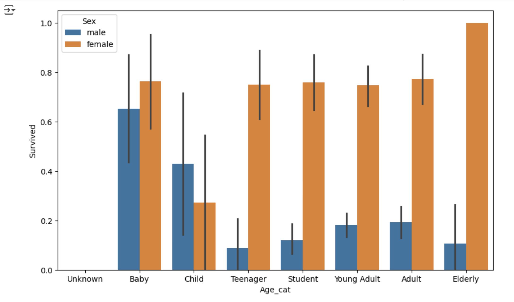

• 여자 Baby: 생존 확률 높음
• 여자 Child: 생존 확률 낮음
• 여자 Elderly: 생존 확률 매우 높음
• Sex, Age, Pclass가 생존에 중요한 피처임을 확인
• 문자열 카테고리 피처 → 숫자형으로 변환 예정
• LabelEncoder 클래스로 레이블 인코딩 적용
• LabelEncoder: 카테고리 값 → 0 ~ (유형 수 - 1) 로 변환
• 대부분의 인코딩은 fit(), transform() 방식
• 여러 칼럼을 한 번에 변환하는 encode_features() 함수 생성 예정

from sklearn.preprocessing import LabelEncoder
def encode_features(dataDF):
  features = ['Cabin', 'Sex', 'Embarked']
  for feature in features:
    le = LabelEncoder( )
    le = le.fit(dataDF[feature])
  dataDF [feature] = le.transform(dataDF[feature])
  return dataDF
titanic_df = encode_features(titanic_df)
titanic_df.head()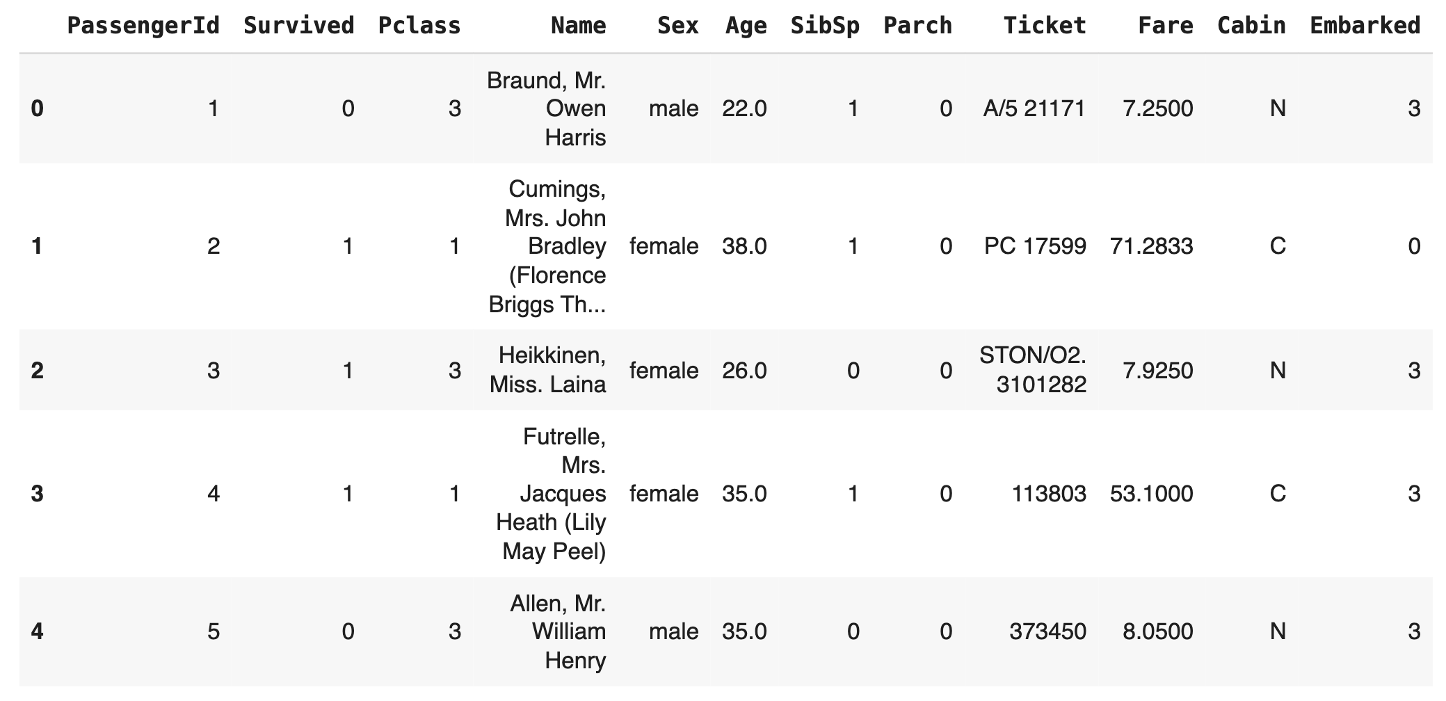

• Sex, Cabin, Embarked 속성이 숫자형으로 변환됨
• 지금까지의 피처 가공 과정을 함수로 정리하여 재사용 가능하도록 구성
• 전체 전처리를 수행하는 함수: transform_features()
• 내부 함수 구성:
  Null 처리
  불필요한 피처 제거 → drop_features(df)
  인코딩 수행
• 제거 대상 피처 (머신러닝 알고리즘에 불필요한 식별자 수준의 피처):
  PassengerId, Name, Ticket

# Null 처리 함수
def fillna(df):
  df['Age'].fillna(df['Age'].mean(), inplace=True)
  df['Cabin'].fillna('N', inplace=True)
  df['Embarked'].fillna('N', inplace=True)
  df['Fare'].fillna(0, inplace=True)
  return df
# 머신러닝 알고리즘에 불필요한 피처 제거
def drop_features (df):
  df.drop(['PassengerId', 'Name', 'Ticket'], axis=1, inplace=True)
  return df
# 레이블 인코딩 수행.
def format_features(df):
  df['Cabin'] = df['Cabin'].str[:1]
  features = ['Cabin', 'Sex', 'Embarked']
  for feature in features:
    le = LabelEncoder()
    le = le.fit(df[feature])
    df[feature] = le.transform(df[feature])
  # Removed premature return statement
  return df # The return statement was inside the for loop, causing it to exit after the first iteration.
# 앞에서 설정한 데이터 전처리 함수 호출
def transform_features(df):
  df = fillna(df)
  df = drop_features(df)
  df = format_features(df)
  return df

• transform_features() 함수로 원본 데이터를 다시 가공함
• CSV 파일을 로딩하고 Survived 속성을 분리해 클래스 결정값 데이터 세트를 생성함
• Survived를 드롭해 피처 데이터 세트를 만들고, transform_features()를 적용함

# 원본 데이터를 재로딩하고 , 피처 데이터 세트와 레이블 데이터 세트 추출.
import pandas as pd
titanic_df = pd.read_csv('sample_data/train.csv')
y_titanic_df = titanic_df['Survived']
X_titanic_df= titanic_df.drop('Survived', axis=1)
X_titanic_df = transform_features(X_titanic_df)

• 내려받은 학습 데이터 세트를 기반으로 해서 train_test_split() API 를 이용해 별도의 테스트 데이터 세트를 추출 -> 테스트 데이터 세트 크기는 전체의 20%

from sklearn.model_selection import train_test_split
X_train, X_test, y_train, y_test=train_test_split(X_titanic_df, y_titanic_df,
                                                  test_size=0.2, random_state=11)

• 결정 트리, 랜덤 포레스트, 로지스틱 회귀를 사용해 타이타닉 생존자 예측 수행함
• DecisionTreeClassifier, RandomForestClassifier, LogisticRegression 클래스를 사용함
• train_test_split()으로 데이터를 나누고, fit으로 학습 후 predict로 예측함
• 정확도 평가는 accuracy_score()로 수행함
• random_state=11은 동일 결과 출력을 위한 설정이며 실제 사례에서는 생략 가능
• solver='liblinear' 는 작은 데이터 세트에서 성능이 좋은 로지스틱 회귀 최적화 알고리즘 설정임

from sklearn.tree import DecisionTreeClassifier
from sklearn.ensemble import RandomForestClassifier
from sklearn.linear_model import LogisticRegression
from sklearn.metrics import accuracy_score

# 분류기 생성
dt_clf = DecisionTreeClassifier(random_state=11)
rf_clf = RandomForestClassifier(random_state=11)
lr_clf = LogisticRegression(solver='liblinear')

# DecisionTreeClassifier 학습 / 예측 / 평가
dt_clf.fit(X_train, y_train)
dt_pred = dt_clf.predict(X_test)
print('DecisionTreeClassifier 정확도 : {:.4f}'.format(accuracy_score(y_test, dt_pred)))

# RandomForestClassifier 학습 / 예측 / 평가
rf_clf.fit(X_train, y_train)
rf_pred = rf_clf.predict(X_test)
print('RandomForestClassifier 정확도 : {:.4f}'.format(accuracy_score(y_test, rf_pred)))

# LogisticRegression 학습 / 예측 / 평가
lr_clf.fit(X_train, y_train)
lr_pred = lr_clf.predict(X_test)
print('LogisticRegression 정확도 : {:.4f}'.format(accuracy_score(y_test, lr_pred)))

• LogisticRegression이 다른 알고리즘보다 높은 정확도를 보임
• 최적화 및 데이터 양이 충분하지 않아 성능 비교는 아직 이름
• 교차 검증으로 결정 트리 모델을 추가 평가함
• KFold, cross_val_score(), GridSearchCV를 사용함
• KFold 클래스는 폴드 개수를 5개로 설정해 사용함

from sklearn.model_selection import KFold
def exec_kfold(clf, folds=5):
# 폴드 세트를 5 개인 KFold 객체를 생성 , 폴드 수만큼 예측결과 저장을 위한 리스트 객체 생성.
  kfold = KFold(n_splits=folds) # Moved this line inside the function
  scores = []
# KFold 교차 검증 수행.
  for iter_count,(train_index, test_index) in enumerate(kfold.split(X_titanic_df)):
# X_titanic_df 데이터에서 교차 검증별로 학습과 검증 데이터를 가리키는 index 생성
    X_train, X_test = X_titanic_df.values[train_index], X_titanic_df.values[test_index]
    y_train, y_test = y_titanic_df.values[train_index], y_titanic_df.values[test_index]
# Classifier 학습 , 예측 , 정확도 계산
    clf.fit(X_train, y_train)
    predictions = clf.predict(X_test)
    accuracy = accuracy_score(y_test, predictions)
    scores.append(accuracy)
    print("교차 검증 {0} 정확도 : {1:.4f}".format(iter_count, accuracy)) # Corrected the format string
# 5개 fold 에서의 평균 정확도 계산.
  mean_score = np.mean(scores)
  print("평균 정확도 : {0:.4f}".format(mean_score))
# exec_kfold 호출
exec_kfold(dt_clf, folds=5)

평균 정확도는 약 78.23% 입니다. 이번에는 교차 검증을 cross_val_score() API 를 이용해 수행합

from sklearn.model_selection import cross_val_score
scores = cross_val_score(dt_clf, X_titanic_df, y_titanic_df, cv=5)
for iter_count, accuracy in enumerate(scores):
  print("교차 검증 {0} 정확도 : {1:.4f}".format(iter_count, accuracy))
  print("평균 정확도 : {0:.4f}".format(np.mean(scores)))

• cross_val_score()는 StratifiedKFold를 사용해 KFold와 평균 정확도에 차이가 있음
• GridSearchCV를 사용해 DecisionTreeClassifier의 최적 하이퍼파라미터를 탐색함
• CV는 5개 폴드로 설정하고, max_depth, min_samples_split, min_samples_leaf를 조정함
• 최적 하이퍼파라미터와 예측 결과를 출력하고, 학습된 Estimator로 테스트 데이터에 대한 예측 정확도를 측정함

from sklearn.model_selection import GridSearchCV
parameters = {'max_depth':[2, 3, 5, 10],
'min_samples_split':[2, 3, 5], 'min_samples_leaf': [1, 5, 8]}
grid_dclf = GridSearchCV(dt_clf, param_grid=parameters, scoring='accuracy', cv=5)
grid_dclf.fit(X_train, y_train)

print('GridSearchcV 최적 하이퍼 파라미터 :', grid_dclf.best_params_)
print('GridsearchcV 최고 정확도 : {0: 4f}'.format(grid_dclf.best_score_))
best_dclf = grid_dclf.best_estimator_
# Gridsearchcv의 최적 하이퍼 파라미터로 학습된 Estimator로 예측 및 평가 수행.
predictions = best_dclf.predict(X_test)
accuracy = accuracy_score(y_test, predictions)
print('테스트 세트에서의 DecisionTreeClassifier 정확도 : (0:.4f)'.format(accuracy))

• 최적 하이퍼파라미터 max_depth=3, min_samples_leaf=5, min_samples_split=2로 학습한 결과 예측 정확도가 약 87.15%로 향상됨
• 하이퍼파라미터 변경 전보다 약 8% 증가했으나, 일반적으로 이 정도 향상은 드물며
• 테스트 데이터 세트가 작아 수치상 성능이 과대평가된 것처럼 보일 수 있음

7. 정리

• 사이킷런은 다양한 ML 알고리즘, 직관적인 API, 편리한 모듈 지원으로 파이썬 대표 ML 패키지임
• 머신러닝은 전처리 → 데이터 분리 → 학습 → 예측 → 평가의 과정으로 구성됨
• 전처리는 오류 보정, Null 처리, 인코딩, 스케일링/정규화 등을 포함함
• 학습 후에는 반드시 별도의 테스트 데이터로 평가해야 하며, 테스트 세트에 치우친 모델 방지를 위해 교차 검증이 필요함
• 사이킷런은 KFold, StratifiedKFold, cross_val_score(), GridSearchCV 등 다양한 교차 검증 도구 제공
• 사이킷런은 안정성과 유용성이 검증된 필수 패키지로, 파이썬 기반 머신러닝 학습에 꼭 필요함
  = 다음 장에서는 분류(Classification)의 예측 성능 평가 방법을 학습함