To . . 언니 🐼 저오늘도열심히썼어여!!칭찬해주세야!~!~!~!~!❤️

🗃️ 다중분류

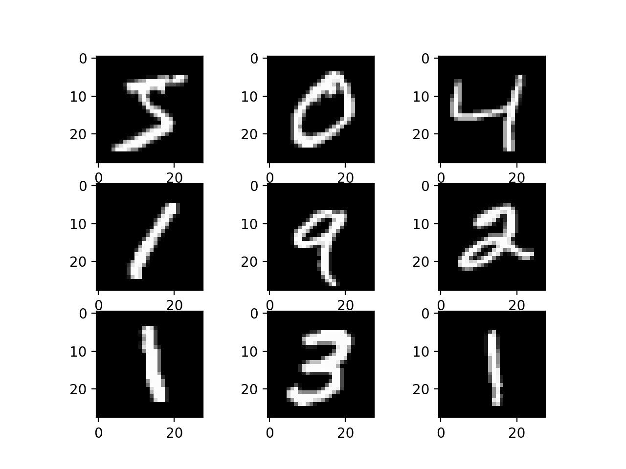
✏️ MNIST 0에서 9까지 숫자 예측

• 과거 NIST에서 수집한 손으로 직접 쓴 흑백숫자
• 데이터는 숫자 이미지(28, 28)와 숫자에 해당하는 레이블로 구성되어 있음
  

---

MNIST 데이터 준비하기

from keras.datasets.mnist import load_data

# Keras 저장소에서 데이터 다운
(X_train, y_train), (X_test, y_test) = load_data(path='mnist.npz')

데이터 형태 확인하기

X_train.shape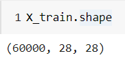

• 

---

# 훈련 데이터
print(X_train.shape, y_train.shape)
print(y_train)

# 테스트 데이터
print(X_test.shape, y_test.shape)
print(y_test)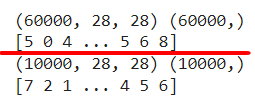

• 

---

데이터 그려보기

import matplotlib.pyplot as plt
import numpy as np

idx = 0
img = X_train[idx, :]
label = y_train[idx]
plt.figure()
plt.imshow(img)
plt.title('%d-th data, label is %d' %(idx, label))

검증 데이터 만들기

from sklearn.model_selection import train_test_split

# 훈련/검증 데이터를 70/30 비율로 분리
X_train, X_val, y_train, y_val = train_test_split(X_train, y_train, test_size=0.3, random_state=777)
print(X_train.shape) # 훈련데이터 42000
print(X_val.shape) # 검증데이터 18000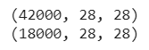

데이터 전처리

모델 입력을 위한 학습데이터(손글씨 이미지 벡터) 전처리

1. 2차원 배열 -> input_dim -> 1차원 배열(28*28=784)
2. 정규화 -> 0 ~ 255 -> 0 ~ 1

1차원 배열로 만들기

num_x_train = X_train.shape[0] # 42000
num_x_val = X_val.shape[0] # 18000
num_x_test = X_test.shape[0] # 10000

# 1. (28, 28) -> 1차원 배열로 처리
X_train = (X_train.reshape(num_x_train, 28*28))
X_val = (X_val.reshape(num_x_val, 28*28))
X_test = (X_test.reshape(num_x_test, 28*28))

print(X_train.shape) -> (42000, 784)
print(X_val.shape) -> (18000, 784)
print(X_test.shape) -> (10000, 784)

정규화 -> 스케일링

여러가지 전처리 방법 - 스케일링

Normalization(MinMax)
Robust Normalization
Standardization

# MinMax 0~255 -> 0~1
X_train = X_train / 255
X_val = X_val / 255
X_test = X_test / 255

print(X_train[0])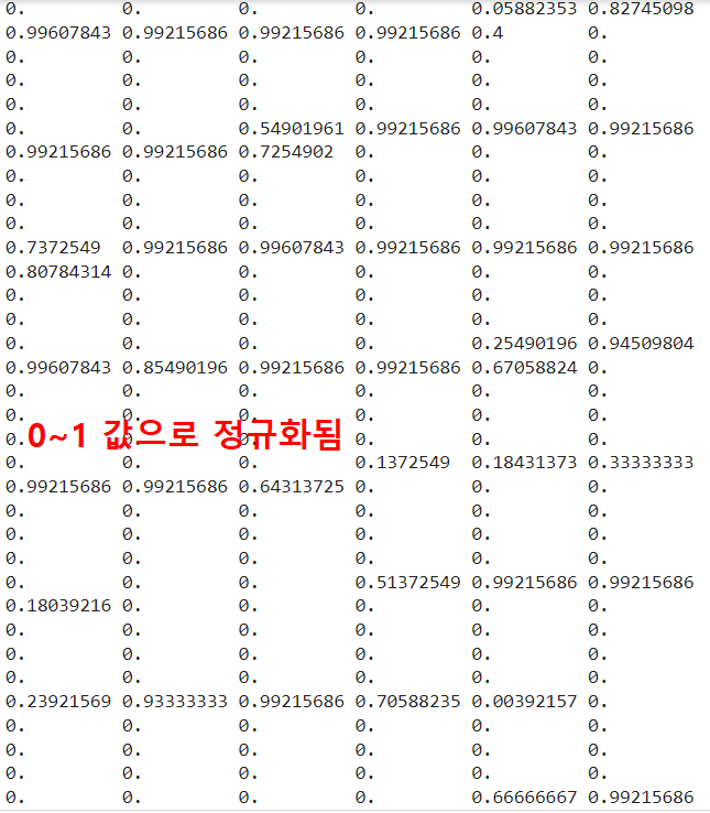

---

모델 입력을 위한 레이블(정답) 전처리

from tensorflow.keras.utils import to_categorical

# 수치 정답 데이터 -> 범주형 데이터로 변경
y_train = to_categorical(y_train)
y_val = to_categorical(y_val)
y_test = to_categorical(y_test)

y_train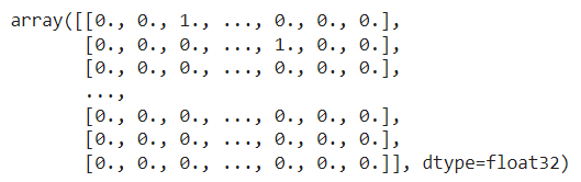

모델 마지막 층에서 소프트맥스(softmax) 함수를 사용하므로 범주형 레이블로 변환

모델 구성하기

from keras.models import Sequential
from keras.layers import Dense

model = Sequential()
model.add(Dense(64, activation='relu', input_dim=784))
model.add(Dense(32, activation='relu'))
# 이중분류 sigmoid 다중분류 softmax
model.add(Dense(10, activation='softmax')) # 10개의 출력을 가진 신경망 -> 정답의 shape와 동일

• 소프트맥스 함수는 출력값의 범위 안에서 확률로써 해석할 수 있기 때문에 결과의 해석이 더욱 용이함
  -> 다른 표현 : 일반적으로 확률을 구하는 방식과 비슷하므로 각 클래스에 해당하는 값들이 서로 영향을 줄 수 있어 비교에 용이
  

모델 설정하기

model.compile(optimizer='adam',loss='categorical_crossentropy', metrics=['acc']) 

모델 학습하기

history = model.fit(X_train, y_train, epochs=30, batch_size=128, validation_data=(X_val, y_val))

학습결과 그리기

import matplotlib.pyplot as plt

his_dict = history.history
loss = his_dict['loss']
val_loss = his_dict['val_loss'] # 검증 데이터가 있는 경우 ‘val_’ 수식어가 붙습니다.

epochs = range(1, len(loss) + 1)
fig = plt.figure(figsize = (10, 5))

# 훈련 및 검증 손실 그리기
ax1 = fig.add_subplot(1, 2, 1)
ax1.plot(epochs, loss, color = 'blue', label = 'train_loss')
ax1.plot(epochs, val_loss, color = 'orange', label = 'val_loss')
ax1.set_title('train and val loss')
ax1.set_xlabel('epochs')
ax1.set_ylabel('loss')
ax1.legend()

acc = his_dict['acc']
val_acc = his_dict['val_acc']

# 훈련 및 검증 정확도 그리기
ax2 = fig.add_subplot(1, 2, 2)
ax2.plot(epochs, acc, color = 'blue', label = 'train_acc')
ax2.plot(epochs, val_acc, color = 'orange', label = 'val_acc')
ax2.set_title('train and val acc')
ax2.set_xlabel('epochs')
ax2.set_ylabel('loss')
ax2.legend()

plt.show()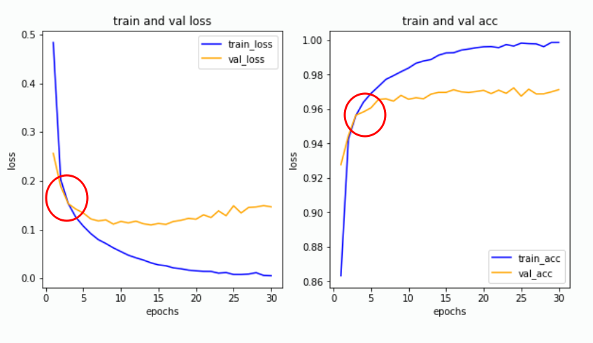

두 그래프가 어디서부터 벌어지는가?

• 과대적합 문제가 나타난 것
• 데이터 특성, 모델 구조 등을 수정해보고 재학습
• 벌어지기 전까지 모델을 사용하여 결과를 확인하고 이를 저장 및 기록

---

모델 평가하기

model.evaluate(X_test, y_test)

• 

---

예측값 그려서 확인

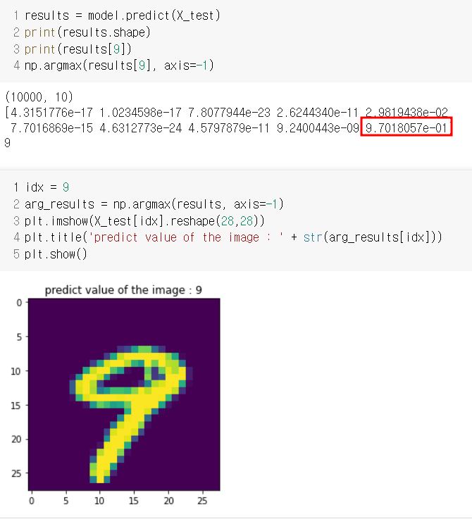
results = model.predict(X_test)
print(results.shape)
print(results[5])
np.argmax(results[5], axis=-1)

idx = 5
arg_results = np.argmax(results, axis=-1)
plt.imshow(X_test[idx].reshape(28,28))
plt.title('predict value of the image : ' + str(arg_results[idx]))
plt.show()

results[9] , idx = 9로 변경하면

0~9까지 값 중 9가 가장 크므로 9로 예측

---

모델 평가

1) 혼동행렬

• 알고리즘이나 모델의 성능을 평가할 때 사용
• 데이터에 대한 모델의 강점과 약점 파악에 유용

from sklearn.metrics import classification_report, confusion_matrix
import seaborn as sns

plt.figure(figsize=(7,7))
cm = confusion_matrix(np.argmax(y_test, axis=-1), np.argmax(results, axis=-1)) # 실제 정답과 비교
sns.heatmap(cm, annot=True, fmt='d', cmap='Blues')
plt.xlabel('predicted label')
plt.ylabel('true label')
plt.show()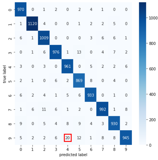

👀 4와 9를 분류할 때 혼란스러워 함

2) 분류 보고서

print(classification_report(np.argmax(y_test, axis=-1), np.argmax(results, axis=-1)))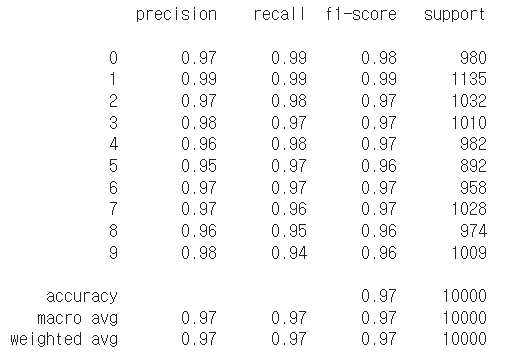

---

📌 주말목표
딥러닝 입문 책보고 배운곳까지 정리해보거나 모르는 부분 이해하기 @ @!

• 과대적합, 과소적합
• 분류 보고서
• 코드분석

이번주에이해못하면프로젝트죽음,,,,,,