Fashion-MNIST 데이터셋

• 60000개 학습 데이터, 10000개 테스트 데이터
  
• Tshirts&top, Trouser, Pullover, Dress, Coat, Sandal, Shirt, Sneaker, Bag, Ankle boot
• 비교를 위한 두가지 모델 구성
  -> (28,28) => 784 대신 Flatten()층 사용

---

데이터 준비하기

from keras.datasets.fashion_mnist import load_data

(X_train, y_train), (X_test, y_test) = load_data()
print(X_train.shape, X_test.shape)

데이터 그려보기

import matplotlib.pyplot as plt
import numpy as np
np.random.seed(777)

class_names = ['T-shirt/top', 'Trouser', 'Pullover', 'Dress', 'Coat', 'Sandal', 'Shirt', 'Sneaker','Bag','Ankle boot']
sample_size = 9
random_idx = np.random.randint(60000, size=sample_size)

plt.figure(figsize=(5,5))
for i, idx in enumerate(random_idx):
  plt.subplot(3,3,i+1)
  plt.xticks([])
  plt.yticks([])
  plt.imshow(X_train[idx], cmap='gray')
  plt.xlabel(class_names[y_train[idx]])
plt.show()

전처리 및 검증 데이터셋 만들기

1) 값의 범위를 0 ~ 255 -> 0 ~ 1 사이로 스케일링(MinMax 알고리즘 사용)

X_train = X_train / 255
X_test = X_test / 255

2) 실제 정답을 비교할 수 있는(다중분류) -> 수치형을 범주형으로 변경

from tensorflow.keras.utils import to_categorical
# 실제 정답 비교를 위해 0 ~ 9 정답지를 따로 저장
real_y_test = y_test

# 레이블 데이터를 범주형으로 변경
y_train = to_categorical(y_train)
y_test = to_categorical(y_test)

3) 훈련 / 검증 데이터를 70:30 비율로 분리

# 3) 훈련 / 검증 데이터를 70:30 비율로 분리
from sklearn.model_selection import train_test_split
X_train, X_val, y_train, y_val = train_test_split(X_train, y_train, test_size=0.3, random_state=777)
X_train.shape

• 

---

• 손실값이 높아지려고 함 -> 정답에서 멀어짐
• 딥러닝에서 깊게 층을 만드는게 무조건 좋은건 아님
• 일반화된 모델을 만드는 것이 중요
• 데이터에 맞는 모델 만들어야

---

첫번째 모델 구성

from keras.models import Sequential
from keras.layers import Dense, Flatten

first_model = Sequential()
first_model.add(Flatten(input_shape=(28,28))) # Flatten(28,28) -> (28*28) -> 1차원 784로 변환
first_model.add(Dense(64, activation='relu'))
first_model.add(Dense(32, activation='relu'))
first_model.add(Dense(10, activation='softmax'))

첫번째 모델 설정

first_model.compile(optimizer='adam', loss='categorical_crossentropy', metrics=['acc'])

첫번째 모델 학습

first_history = first_model.fit(X_train, y_train, epochs=30, batch_size=128, validation_data=(X_val, y_val))

---

두번째 모델

from keras.models import Sequential
from keras.layers import Dense, Flatten

second_model = Sequential()
second_model.add(Flatten(input_shape=(28,28))) # Flatten(28,28) -> (28*28) -> 1차원 784로 변환
second_model.add(Dense(128, activation='relu')) # 층 하나 추가
second_model.add(Dense(64, activation='relu'))
second_model.add(Dense(32, activation='relu'))
second_model.add(Dense(10, activation='softmax'))

second_model.compile(optimizer='adam', loss='categorical_crossentropy', metrics=['acc'])

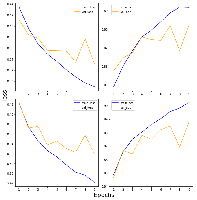
second_history = second_model.fit(X_train, y_train, epochs=30, batch_size=128, validation_data=(X_val, y_val))

---

학습 결과 그리기

import numpy as np
import matplotlib.pyplot as plt

def draw_loss_acc(history_1, history_2, epochs):
    his_dict_1 = history_1.history
    his_dict_2 = history_2.history
    keys = list(his_dict_1.keys())
    
    epochs = range(1, epochs)
    fig = plt.figure(figsize = (10, 10))
    ax = fig.add_subplot(1, 1, 1)
    # axis 선과 ax의 축 레이블을 제거합니다.
    ax.spines['top'].set_color('none')
    ax.spines['bottom'].set_color('none')
    ax.spines['left'].set_color('none')
    ax.spines['right'].set_color('none')
    ax.tick_params(labelcolor='w', top=False, bottom=False, left=False, right=False)
    
    for i in range(len(his_dict_1)):
        temp_ax = fig.add_subplot(2, 2, i + 1)
        temp = keys[i%2]
        val_temp = keys[(i + 2)%2 + 2]
        temp_history = his_dict_1 if i < 2 else his_dict_2
        temp_ax.plot(epochs, temp_history[temp][1:], color = 'blue', label = 'train_' + temp)
        temp_ax.plot(epochs, temp_history[val_temp][1:], color = 'orange', label = val_temp)
        if(i == 1 or i == 3):
            start, end = temp_ax.get_ylim()
            temp_ax.yaxis.set_ticks(np.arange(np.round(start, 2), end, 0.01))
        temp_ax.legend()
    ax.set_ylabel('loss', size = 20)
    ax.set_xlabel('Epochs', size = 20)
    plt.tight_layout()
    plt.show()
    
draw_loss_acc(first_history, second_history, 30)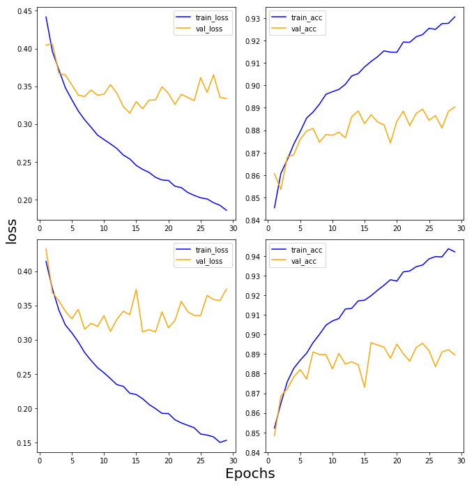

모델 평가

first_model.evaluate(X_test, y_test)
second_model.evaluate(X_test, y_test)

• 

---

학습 횟수 10으로 조정

---

모델 예측하여 그려보기

import numpy as np

results = first_model.predict(X_test)
arg_results = np.argmax(results, axis = -1)

random_idx = np.random.randint(10000)

plt.figure(figsize=(5,5))

plt.imshow(X_test[random_idx], cmap='gray')
plt.title('Predicted value of the image : ' + class_names[arg_results[random_idx]] + ', Real value of the image :' + class_names[real_y_test[random_idx]])
plt.show()

• 틀린경우
• 맞은경우

---

모델 평가 - 혼동행렬

from sklearn.metrics import classification_report, confusion_matrix
import seaborn as sns
results = first_model.predict(X_test)

plt.figure(figsize=(7,7))

cm = confusion_matrix(np.argmax(y_test, axis=-1), np.argmax(results, axis=-1)) # 실제 정답과 비교
sns.heatmap(cm, annot=True, fmt='d', cmap='Blues')
plt.xlabel('predicted label')
plt.ylabel('true label')
plt.show()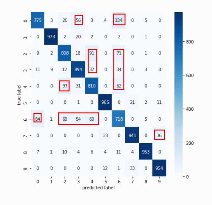

---

결과 해석

• 모델을 깊게 구성 -> 높은 성능, But 과대적합(파라미터 수 증가)
• 모델의 깊이는 데이터에 적합하게 결정해야 함
• 유명한 데이터셋이나 유사 분야에서 높은 성능을 보여준 모델 구조를 참고하여 구성해보고 실험 진행