머신러닝 - Bike Sharing Demand

https://www.kaggle.com/competitions/bike-sharing-demand

Data Fields
datetime  hourly date + timestamp
season -  1 = spring, 2 = summer, 3 = fall, 4 = winter 
holiday - whether the day is considered a holiday
workingday - whether the day is neither a weekend nor holiday
weather 
- 1: Clear, Few clouds, Partly cloudy, Partly cloudy
2: Mist + Cloudy, Mist + Broken clouds, Mist + Few clouds, Mist
3: Light Snow, Light Rain + Thunderstorm + Scattered clouds, Light Rain + Scattered clouds
4: Heavy Rain + Ice Pallets + Thunderstorm + Mist, Snow + Fog 
temp - temperature in Celsius
atemp - "feels like" temperature in Celsius
humidity - relative humidity
windspeed - wind speed
casual - number of non-registered user rentals initiated
registered - number of registered user rentals initiated
count - number of total rentals

데이터셋

train = pd.read_csv("data/bike/train.csv")
print(train.shape)
train.head(2)

(10886, 12)

test = pd.read_csv("data/bike/test.csv")
print(test.shape)
test.head(2)

(6493, 9)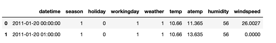

# train에만 있는 columns
set(train.columns) - set(test.columns)

{'casual', 'count', 'registered'}

train.info()
<class 'pandas.core.frame.DataFrame'>
RangeIndex: 10886 entries, 0 to 10885
Data columns (total 12 columns):
 #   Column      Non-Null Count  Dtype  
---  ------      --------------  -----  
 0   datetime    10886 non-null  object 
 1   season      10886 non-null  int64  
 2   holiday     10886 non-null  int64  
 3   workingday  10886 non-null  int64  
 4   weather     10886 non-null  int64  
 5   temp        10886 non-null  float64
 6   atemp       10886 non-null  float64
 7   humidity    10886 non-null  int64  
 8   windspeed   10886 non-null  float64
 9   casual      10886 non-null  int64  
 10  registered  10886 non-null  int64  
 11  count       10886 non-null  int64  
dtypes: float64(3), int64(8), object(1)
memory usage: 1020.7+ KB

test.info()
<class 'pandas.core.frame.DataFrame'>
RangeIndex: 6493 entries, 0 to 6492
Data columns (total 9 columns):
 #   Column      Non-Null Count  Dtype  
---  ------      --------------  -----  
 0   datetime    6493 non-null   object 
 1   season      6493 non-null   int64  
 2   holiday     6493 non-null   int64  
 3   workingday  6493 non-null   int64  
 4   weather     6493 non-null   int64  
 5   temp        6493 non-null   float64
 6   atemp       6493 non-null   float64
 7   humidity    6493 non-null   int64  
 8   windspeed   6493 non-null   float64
dtypes: float64(3), int64(5), object(1)
memory usage: 456.7+ KB

# 결측치 확인
train.isnull().sum().sum()

0

test.isnull().sum()

datetime      0
season        0
holiday       0
workingday    0
weather       0
temp          0
atemp         0
humidity      0
windspeed     0
dtype: int64

train.describe()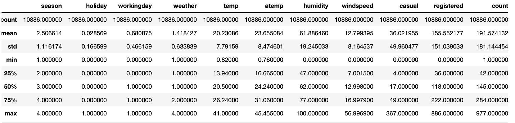

전처리

• 연, 월, 일, 시, 분, 초 만들기

train['datatime] = pd.to_datetime(train['datetime'])
train['year'] = train['datetime'].dt.year
train['month'] = train['datetime'].dt.month
train['day'] = train['datetime'].dt.day
train['hour'] = train['datetime'].dt.hour
train['minute'] = train['datetime'].dt.minute
train['second'] = train['datetime'].dt.second
train.head(2)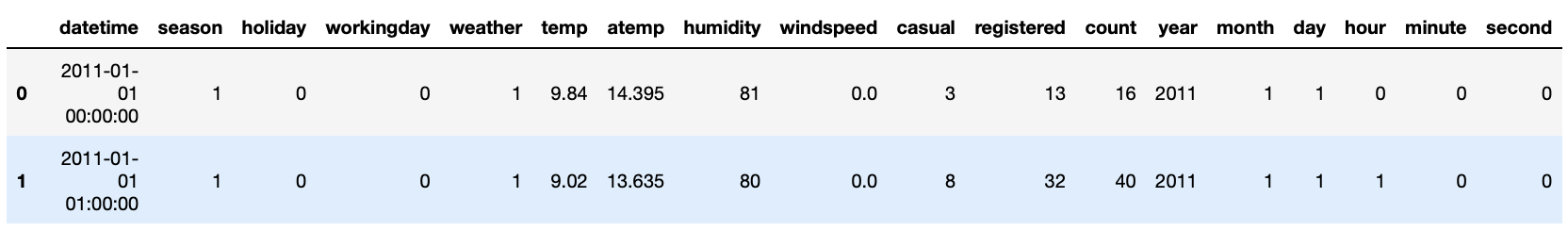

test['datetime'] = pd.to_datetime(test['datetime'])
test['year'] = test['datetime'].dt.year
test['month'] = test['datetime'].dt.month
test['day'] = test['datetime'].dt.day
test['hour'] = test['datetime'].dt.hour
test['minute'] = test['datetime'].dt.minute
test['second'] = test['datetime'].dt.second
test.head(2)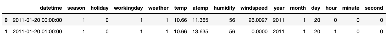

EDA

histograms

train.hist(figsize=(12, 12), bins=50)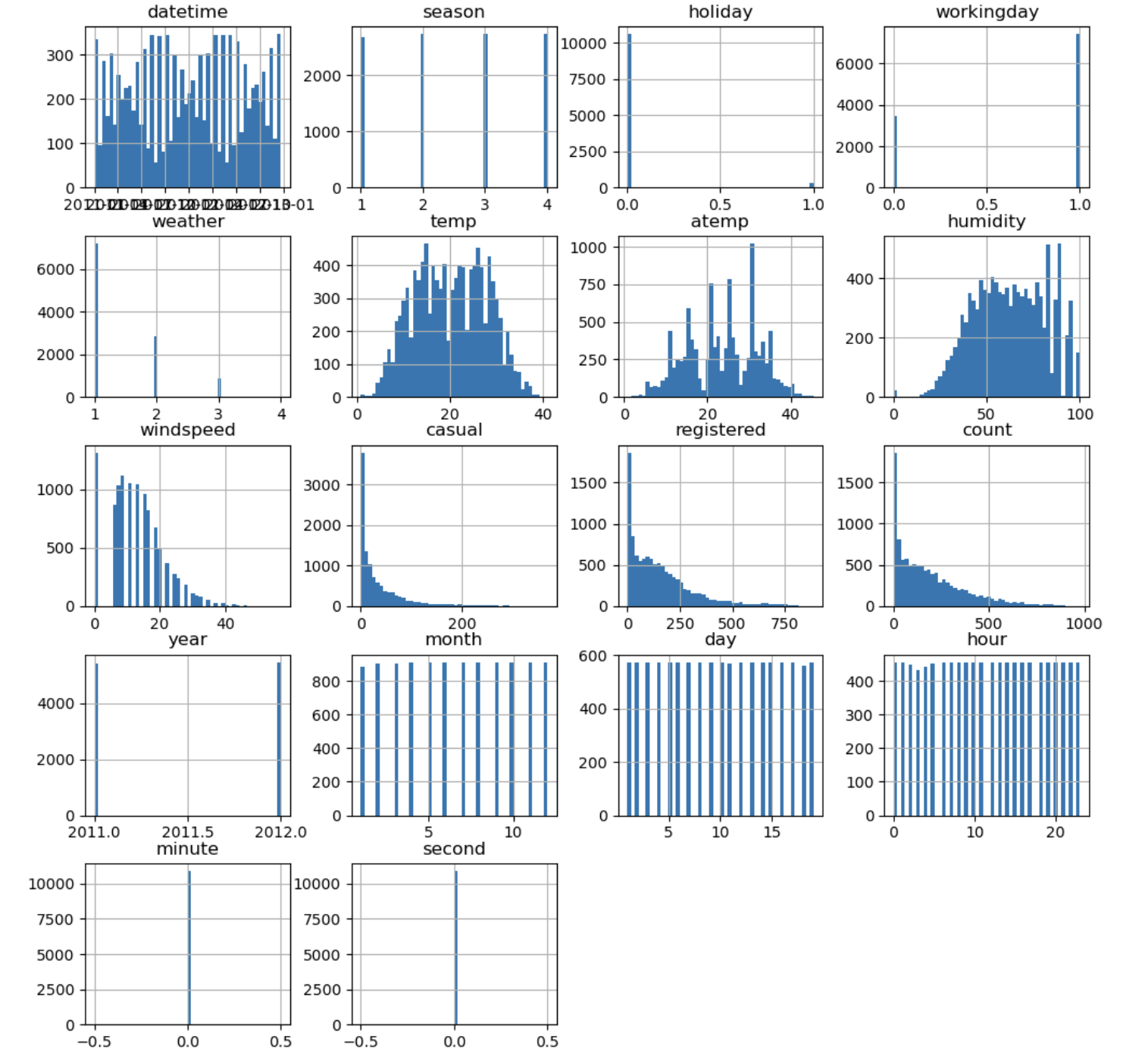

test.hist(figsize=(12, 12), bins=50);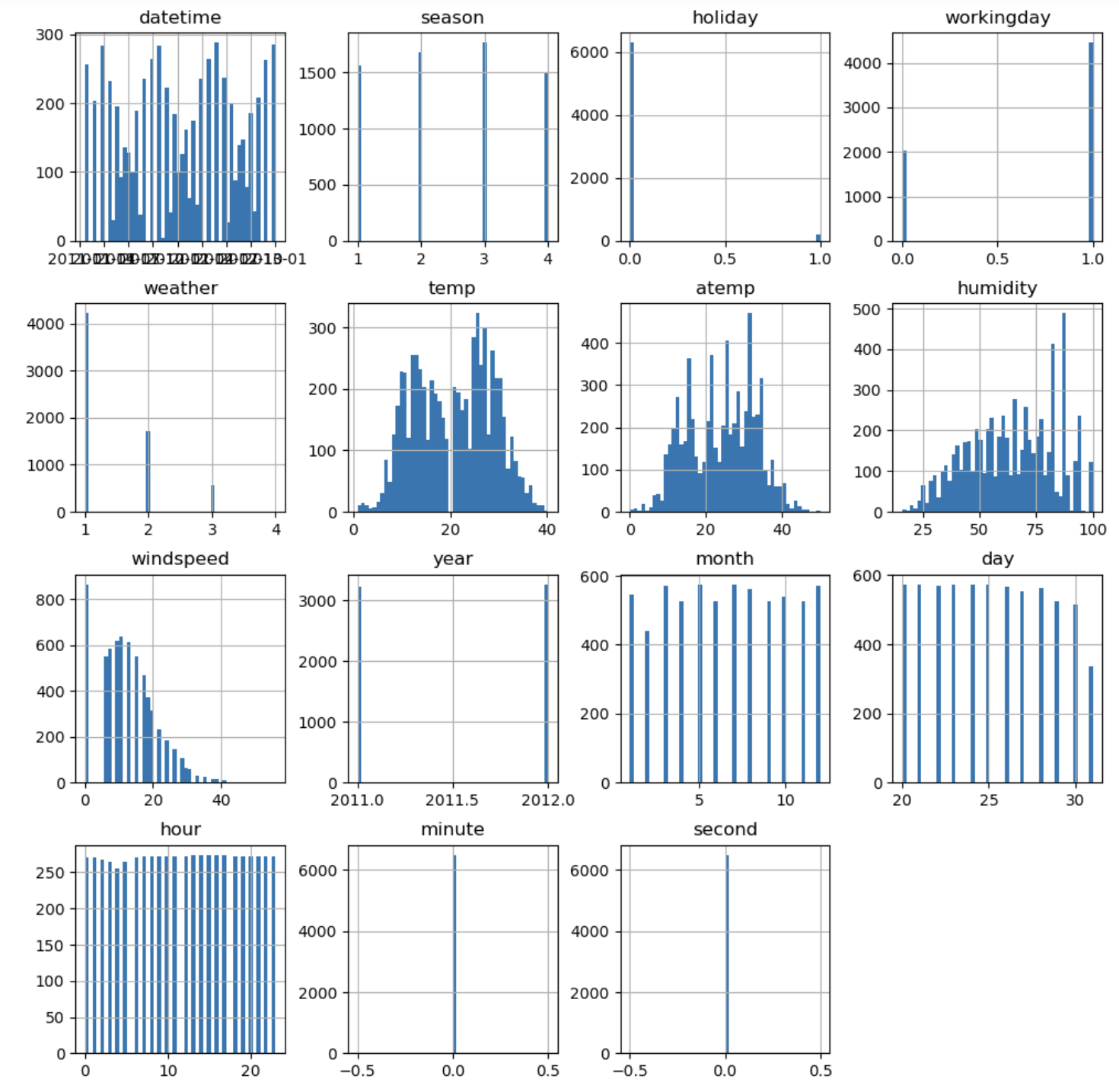

풍속별 자전거 대여량 분포

# 풍속별 자전거 대여량 분포 시각화
sns.scatterplot(data=train, x='windspeed', y='count')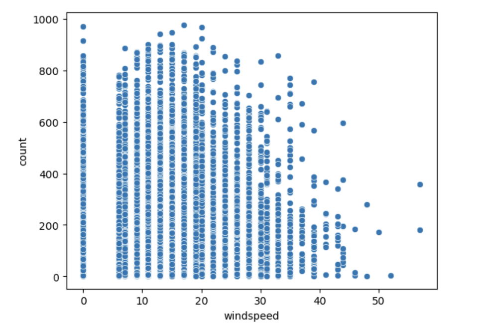

습도별 자전거 대여량 분포

# 습도별 자전거 대여량 분포 시각화
sns.scatterplot(data=train, x='humidity', y='count')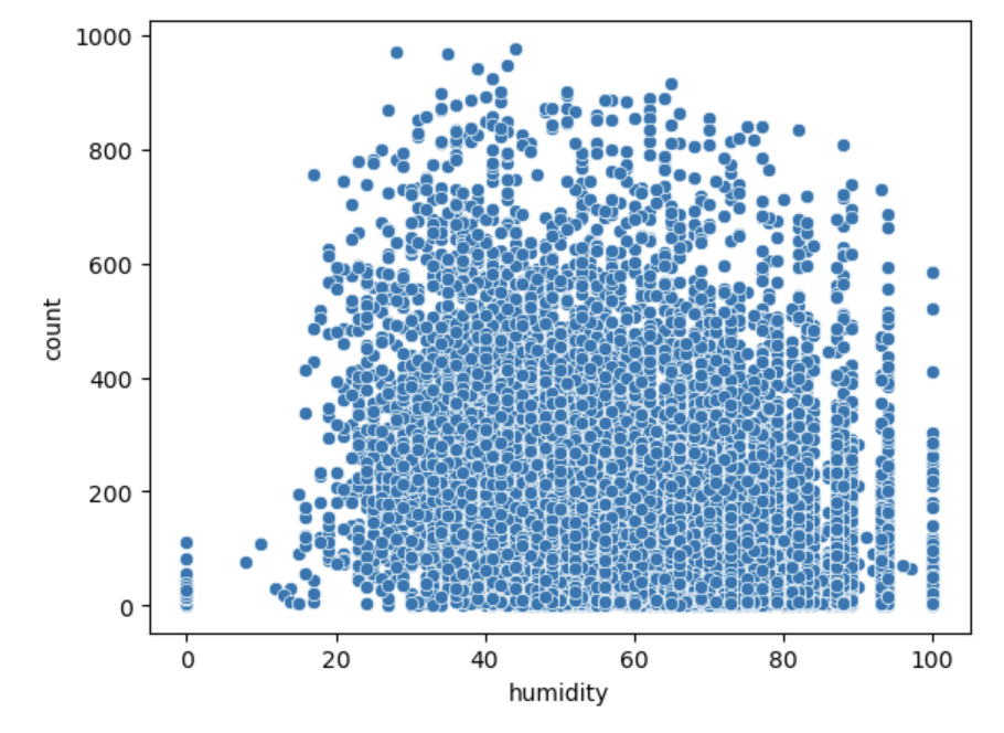

기온별 체감기온 분포

# 기온별 체감기온 분포 시각화
sns.scatterplot(data=train, x='temp', y='atemp')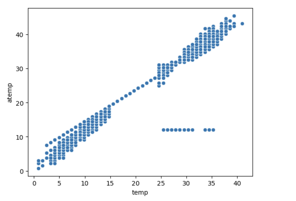

train[(train['temp'] - train['atemp'] > 10)][['temp', 'atemp']].shape
(24, 2)

날씨별 대여수 분포도

# 날씨별 대여수 분포도
sns.barplot(data=train, x='weather', y='count', errorbar=None)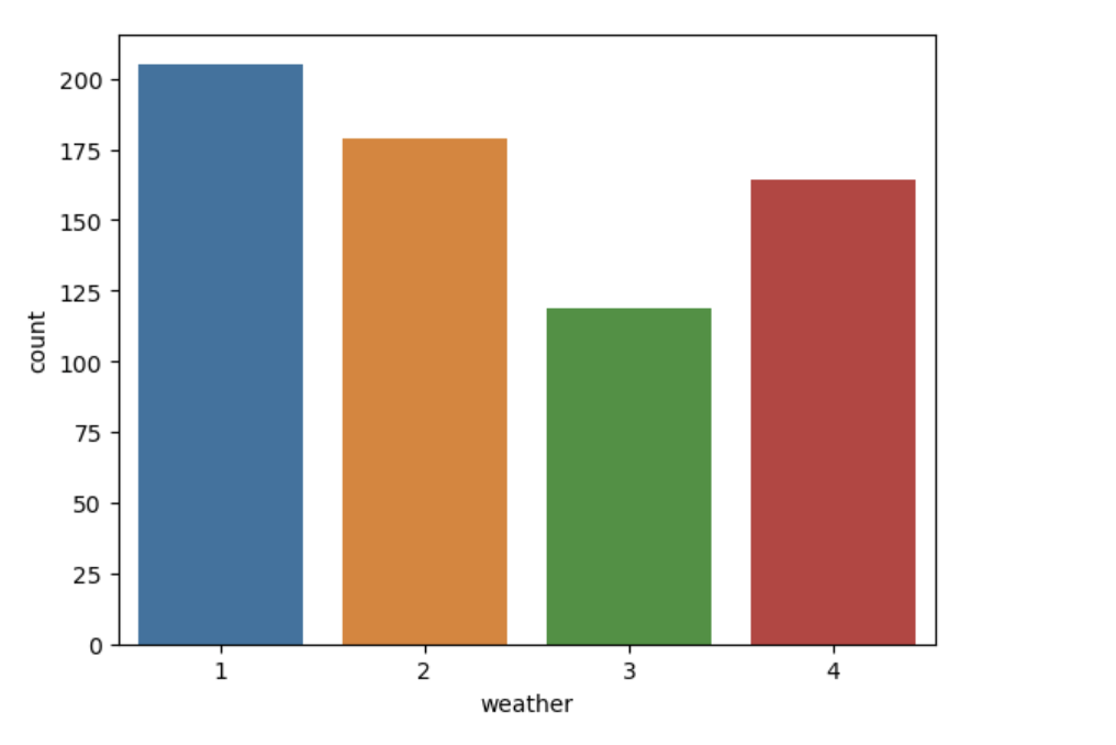

# weather 4 -> 폭우와 폭설이 내린 시간이 많지 않아서 
# 데이터 1개 뿐이라 count 값이 많게 나옴
train[train['weather'] == 4]

날짜별

# day는 train, test 나누는 기준
# train은 19일 까지, test는 20일 부터
# day는 feature에서 제거하는 게 낫다. 
sns.barplot(data=train, x="day", y="count")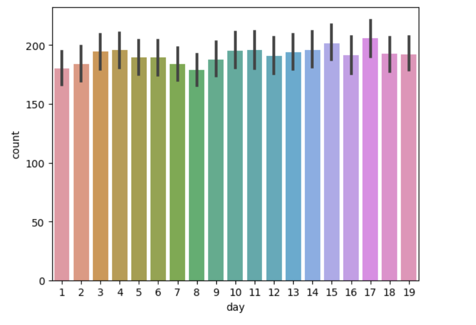

# 월별로 차이가 있어보이고 날씨가 추운 겨울에는 대여량 적고 5-10월에는 대여량 많음. 
sns.barplot(data=train, x='month', y='count)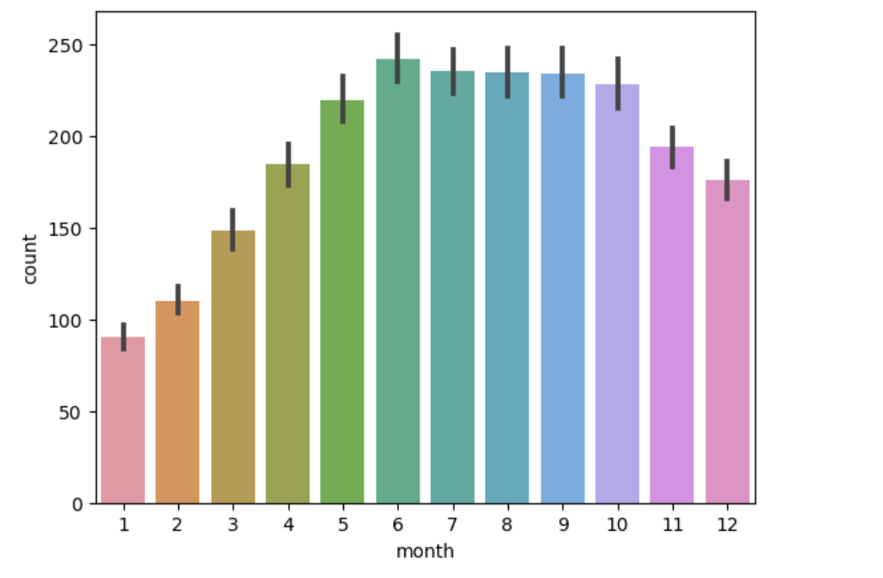

Season

# season별 month 기술통계 
train.groupby('season')['month'].describe()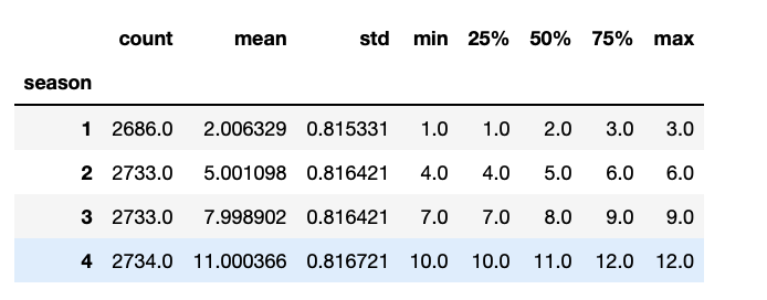

# season의 month 요약
train.groupby('season')['month'].unique()

season
1       [1, 2, 3]
2       [4, 5, 6]
3       [7, 8, 9]
4    [10, 11, 12]
Name: month, dtype: object

sns.barplot(data=train, x='season', y='count', hue='year')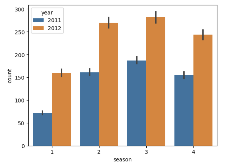

year-month

train['year-month'] = train['datetime].astype(str).str[:7]
test['year-month'] = test['datetime].astype(str).str[:7]

plt.figure(figsize=(24, 3))
sns.barplot(data=train, x="year-month", y='count')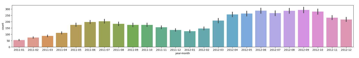

Ordinal-Encoding

• categoty 데이터타입 변경하면 ordinal encoding 가능, 순서O

train['year-month-code'] = train['year-month'].astype('category').cat.codes
test['year-month-code'] = test['year-month'].astype('category').cat.codes

학습, 예측 데이터셋

정답값

label_name = 'count'

학습, 예측 데이터

feature_names = ['hour',
                 'workingday', 'weather', 'temp',
                 'atemp', 'humidity', 'windspeed']

X_train = train[feature_names]
print(X_train.shape)
X_train.head(2)
(10886, 7)

	hour	workingday	weather		temp	atemp	humidity	windspeed
0	0		0			1			9.84	14.395	81			0.0
1	1		0			1			9.02	13.635	80			0.0


X_test = test[feature_names]
print(X_test.shape)
X_test.head(2)
(6493, 7)

	hour	workingday	weather	temp	atemp	humidity	windspeed
0	0		1			1		10.66	11.365	56			26.0027
1	1		1			1		10.66	13.635	56			0.0000


y_train = train[label_name]
print(y_train.shape)
y_train.head(2)
(10886,)

0    16
1    40
Name: count, dtype: int64

머신러닝 알고리즘

RandomForest

# RandomForest
# criterion : {"squared_error", "absolute_error", "poisson"},default="squared_error"
from sklearn.ensemble import RandomForestRegressor
model = RandomForestRegressor(random_state=42, n_jobs=-1)

cross-validation 교차검증

• cross_val_predict : 예측한 predict 값을 반환하여 직접 계산 가능
• 다른 cross_val_score, cross_validate : score을 조각마다 직접 계산

from sklearn.model_selection import cross_val_predict

y_valid_pred = cross_val_predict(model, X_train, y_train, cv=5, n_jobs=-1, verbose=2)
y_valid_pred

array([ 99.685     ,  80.55166667,  50.75905556, ..., 141.54      ,
       107.464     ,  51.52      ])

평가

MAE(Mean Absolute Error)

MAE = abs(y_train - y_valid_pred).mean()

# sklearn 활용
from sklearn.metrics import mean_absolute_error
mean_absolute_error(y_train, y_valid_pred)
>>>>
71.93404282768897

MSE(Mean Squared Error)

MSE = np.square(y_train - y_valid_pred).mean()

# sklearn 활용
from sklearn.metrics import mean_squared_error
mean_squared_error(y_train, y_valid_pred)
>>>>
10858.226980881813

RMSE(Root Mean Squared Error)

RMSE = np.sqrt(MSE)
>>>>
104.20281656885199

RMSLE(Root Mean Squared Logarithmic Error)

sns.kdeplot(y_train)
sns.kdeplot(y_valid_pred)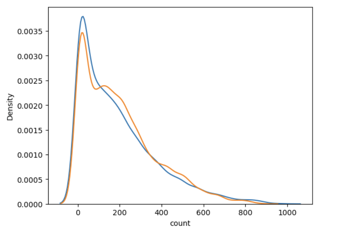

sns.scatterplot(x=y_train, y=y_valid_pred)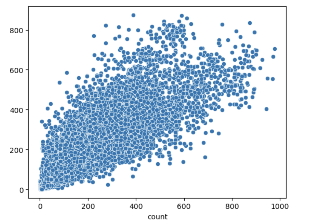

• 정답인 count에 +1 하면 0보다 작은 값이 있을 때 마이너스 무한대로 수렴하는 것 방지
• +1 하고 log

sns.kdeplot(np.log(train['count'] + 1))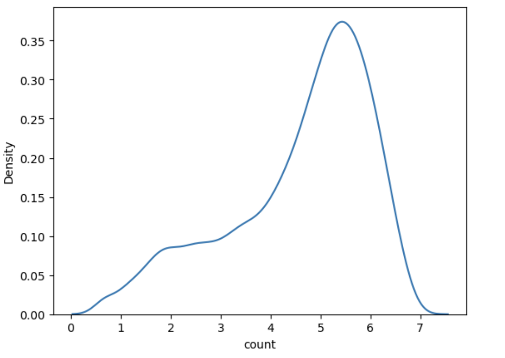

log1p

np.log(train['count'] + 1)

0        2.833213
1        3.713572
2        3.496508
3        2.639057
4        0.693147
           ...   
10881    5.820083
10882    5.488938
10883    5.129899
10884    4.867534
10885    4.488636
Name: count, Length: 10886, dtype: float64

• np.log(x + 1) == np.log1p(x)

np.log1p(y_train).describe()

count    10886.000000
mean         4.591364
std          1.419454
min          0.693147
25%          3.761200
50%          4.983607
75%          5.652489
max          6.885510
Name: count, dtype: float64

RMSLE

• 오차가 작을수록 가중치를 주게 됨 (로그의 효과)

from sklearn.metrics import mean_squared_log_error

RMSLE = np.sqrt(mean_squared_log_error(y_train, y_valid_pred))
RMSLE
>>>>
0.577092112424969

학습과 예측

y_predict = model.fit(X_train, y_train).predict(X_test)

# feature_importances
sns.barplot(x=model.feature_importances_, y=model.feature_names_in_)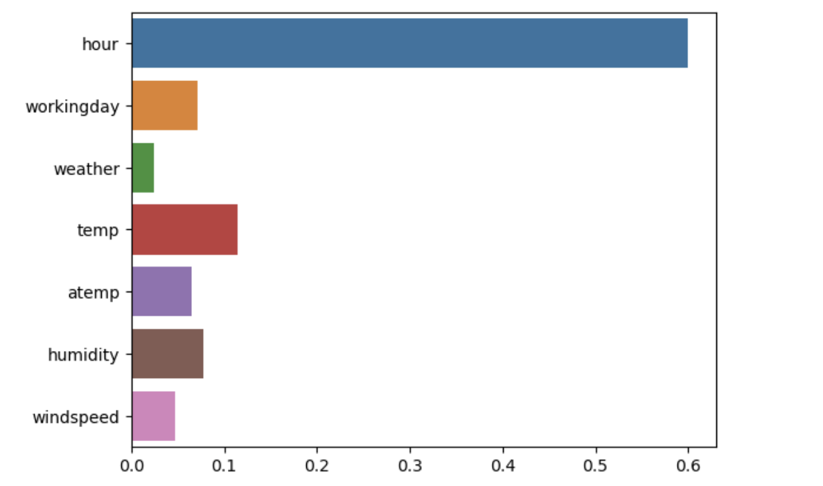

kaggle submission

# 답안지 양식 불러오기
submit = pd.read_csv("data/bike/samplesubmission.csv")

# 예측한 값을 답안지에 옮겨 적기
submit["count"] = y_predict

file_name = f"data/bike/submit_{RMSLE:.5f}.csv"

# 캐글에 제출하기 위해 csv 파일로 저장합니다.
submit.to_csv(file_name, index=False)

# 파일 저장이 제대로 되었는지 확인합니다.
pd.read_csv(file_name).head(2)