머신러닝 - Bike Sharing Demand (log)

전처리

train['datetime'] = pd.to_datetime(train['datetime'])

train['year'] = train['datetime].dt.year
train["month"] = train["datetime"].dt.month
train["day"] = train["datetime"].dt.day
train["hour"] = train["datetime"].dt.hour
train["minute"] = train["datetime"].dt.minute
train["second"] = train["datetime"].dt.second
train["dayofweek"] = train["datetime"].dt.dayofweek

print(train.shape)
train[['datetime', 'year', 'month', 
       'day', 'hour','minute', 
       'second', "dayofweek"]].head()]]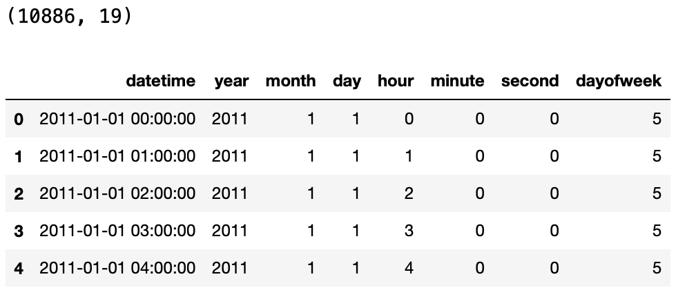

test["datetime"] = pd.to_datetime(test["datetime"])

test["year"] = test["datetime"].dt.year
test["month"] = test["datetime"].dt.month
test["day"] = test["datetime"].dt.day
test["hour"] = test["datetime"].dt.hour
test["minute"] = test["datetime"].dt.minute
test["second"] = test["datetime"].dt.second
test["dayofweek"] = test["datetime"].dt.dayofweek

print(test.shape)
test[['datetime', 'year', 'month', 
       'day', 'hour','minute', 
       'second', 'dayofweek']].head()

EDA

log & exp

• log() + 1 == log1p()
• log에 1 을 더하는 이유 -> 1보다 작은 값은 음수를 갖기 때문에
• 가장 작은 값인 1을 더해 음수가 나오지 않게 하기위하여

train['count_log1p'] = np.log(train['count'] + 1)
train['count_expm1'] = np.exp(train['count_log1p]) -1

# log를 count 값에 적용하게 되면 분포가 완만해짐
# log를 취한 값 사용 -> 이상치에도 덜 민감하게 됨

fig, axes = plt.subplots(nrow=1, ncols=3, figsize=(12, 3))
# count - kdeplot
sns.kdeplot(train['count'], ax=axes[0])
# count log1p - kdeplot
sns.kdeplot(train['count_log1p'], ax=axes[1])
# count expm1 - kdeplot
sns.kdeplot(train['count_expm1'], ax=axes[2])

• np.exp() 지수함수 : np.log() 로그로 취했던 값을 다시 원래 값으로 복원
• count == np.expm1(np.log())
• log : 먼저 + 1 -> log 적용
• exp : 먼저 exp 적용 -> -1 빼준다

train['count_expm1'] = np.exp(train['count_log1p']) -1
train[['count', 'count_log1p', 'count_expm1']].describe()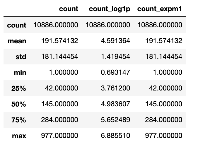

학습 & 예측 데이터

정답값

label_name = 'count_log1p'

feature

train.columns
>>>>
Index(['datetime', 'season', 'holiday', 'workingday', 'weather', 'temp',
       'atemp', 'humidity', 'windspeed', 'casual', 'registered', 'count',
       'year', 'month', 'day', 'hour', 'minute', 'second', 'dayofweek',
       'count_log1p', 'count_expm1'],
      dtype='object')
 
feature_names = ['holiday','workingday', 'weather', 'temp',
       'atemp', 'humidity', 'windspeed', 'year', 'hour', 'dayofweek', 'season' ]

학습 데이터셋

X_train = train[feature_names]
print(X_train.shape)
X_train.head(2)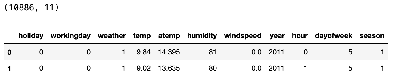

예측 데이터셋

X_test = test[feature_names]
print(X_test.shape)
X_test.head(2)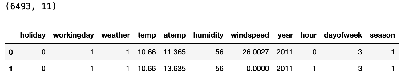

정답값

y_train = train[label_name]
print(y_train.shape)
y_train.head(2)

(10886,)
0    2.833213
1    3.713572
Name: count_log1p, dtype: float64

머신러닝 알고리즘

from sklearn.ensemble import RandomForestRegressor

model = RandomForestRegressor(random_state=42, n_jobs=-1)

GridSearchCV or RandomizedSearchCV

from sklearn.model_selection import RandomizedSearchCV

param_distributions = {"max_depth" : np.random.randint(15, 30, 10), 
						'max_features" : np.random.uniform(0.8, 1, 10)}
reg = RandomizedSearchCV(model, param_distributions=param_distributions,
                         n_iter=10, cv=5, 
                         verbose=2, n_jobs=-1, 
                         random_state=42,
                         scoring = 'neg_root_mean_squared_error')

reg.fit(X_train, y_train)

>>>>
RandomizedSearchCV(cv=5,
                   estimator=RandomForestRegressor(n_jobs=-1, random_state=42),
                   n_jobs=-1,
                   param_distributions={'max_depth': array([23, 15, 15, 24, 22, 25, 20, 27, 22, 25]),
                                        'max_features': array([0.96712523, 0.85946277, 0.84612712, 0.85868195, 0.8458574 ,
       0.89176561, 0.96668001, 0.93522851, 0.99276914, 0.96915596])},
                   random_state=42, scoring='neg_root_mean_squared_error',
                   verbose=2)

best_estimator

reg.best_estimator_
>>>>
RandomForestRegressor(max_depth=25, max_features=0.8586819477840943, n_jobs=-1,
                      random_state=42)

# scoring = 'neg_root_mean_squared_error' -> score 음수로 출력
reg.best_score_
>>>> -0.4459476222346657

rmsle = abs(reg.best_score_)
rmsle
>>>> 0.4459476222346657

best_model = reg.best_estimator_

from sklearn.model_selection import cross_val_predict

y_valid_pred = cross_val_predict(best_model, X_train, y_train,
								cv=5, n_jobs=-1, verbose=2)
y_valid_pred[:5]
>>>>
array([4.29830286, 4.09970921, 3.82383222, 2.86231615, 1.93402827])

평가

MSE(Mean Squared Error)

from sklearn.metrics import mean_squared_error

mean_squared_error(y_train, y_valid_pred)
>>>> 0.21607239024175462

RMSE(Root Mean Squared Error)

mean_squared_error(y_train, y_valid_pred) ** 0.5
>>>> 0.4648358745210557

RMSLE(Root Mean Squared Logarithmic Error)

rmsle = abs(reg.best_score_)
rmsle 
>>>> 0.4459476222346657

학습 & 예측

y_predict = best_model.fit(X_train, y_train).predict(X_test)

# feature_importances
sns.barplot(x=best_model.feature_importances_, y=best_model.feature_names_in_)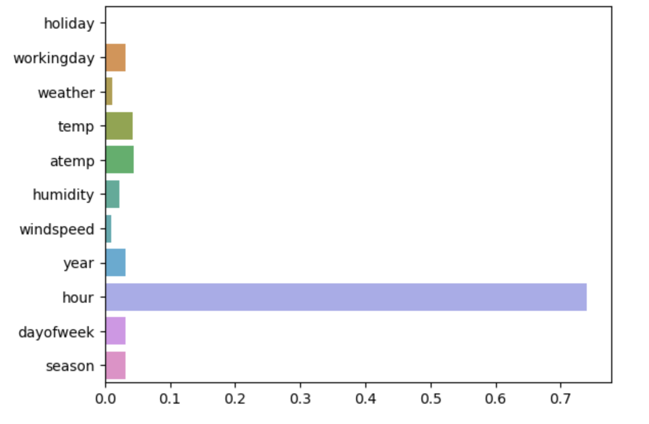

Kaggle Submission

df_submit = pd.read_csv(f"{base_path}/sampleSubmission.csv")

# np.expm1을 count에 적용하는 것 주의
df_submit['count'] = np.expm1(y_predict)

file_name = f"{base_path}/submot{rmsle}.csv"

df_submit.to_csv(file_name, index=False)