머신러닝 - DecisionTree

psy4072·2022년 10월 27일

Classifier pandas plot_tree scikit learn

멋쟁이 사자처럼 AI 스쿨

목록 보기

8/34

Pima Indians Diabetes Database

라이브러리 로드

import pandas as pd
import numpy as np
import seaborn as sns
import matplot.pyplot as plt

데이터셋 로드

df = pd.read_csv("http://bit.ly/data-diabetes-csv")
df.shape
=> (768, 9)

df.head()

	Pregnancies	Glucose	BloodPressure	SkinThickness	Insulin	BMI		DiabetesPedigreeFunction	Age	Outcome
0	6			148		72				35				0		33.6	0.627						50	1
1	1			85		66				29				0		26.6	0.351						31	0
2	8			183		64				0				0		23.3	0.672						32	1
3	1			89		66				23				94		28.1	0.167						21	0
4	0			137		40				35				168		43.1	2.288						33	1

학습과 예측 과정

-feature_names : 학습(훈련), 예측에 사용할 컬럼을 리스트 형태로 만들어서 변수에 담아줍니다.
-label_name : 정답값
-X_train : feature_names 에 해당되는 컬럼만 train에서 가져옵니다.
			학습(훈련)에 사용할 데이터셋 예) 시험의 기출문제
-X_test : feature_names 에 해당되는 컬럼만 test에서 가져옵니다.
			예측에 사용할 데이터셋 예) 실전 시험문제
-y_train : label_name 에 해당 되는 컬럼만 train에서 가져옵니다.
			학습(훈련)에 사용할 정답 값 예) 기출문제의 정답
-model : 학습, 예측에 사용할 머신러닝 알고리즘
-model.fit(X_train, y_train) : 학습(훈련), 기출문제와 정답을 가지고 학습(훈련)하는 과정과 유사합니다.
-model.predict(X_test) : 예측, 실제 시험을 보는 과정과 유사합니다. => 문제를 풀어서 정답을 구합니다.
-score : 시험을 봤다면 몇 문제를 맞고 틀렸는지 채점해 봅니다.
-metric
 : 점수를 채점하는 공식입니다. (예를 들어 학교에서 중간고사를 봤다면 전체 평균을 계산해 줍니다.)

학습과 예측 데이터셋 나누기

# 8:2 비율을 구하기 위해 전체 데이터의 행에서 80% 값
split_count = int(df.shape[0] * 0.8)
split_count
=> 614

# train, test 슬라이싱
train = df[:split_count]
test = df[split_count:]

train.shape, test.shape
=> (614, 9), (154, 9)

학습, 예측에 사용 컬럼

feature_names = df.columns.tolist()
feature_names.remove("Outcome")
feature_names
=>
['Pregnancies',
 'Glucose',
 'BloodPressure',
 'SkinThickness',
 'Insulin',
 'BMI',
 'DiabetesPedigreeFunction',
 'Age']

정답값이자 예측해야 될 값

label_name = "Outcome"

학습, 예측 데이터셋 만들기

X : feature, 독립변수 -> 시험문제
y : label, 종속변수 -> 정답

# 학습 세트
X_train = train[feature_names]
X_train.shape
=> (614, 8)

# 정답 값
y_train = train[label_name]
y_train.shape
=> (614,)

# 예측에 사용할 데이터셋
X_test = test[feature_names]
X_test.shape
=> (154, 8)

# 예측의 정답값
y_test = test[label_name]
y_test.shape
=> (154,)

머신러닝 알고리즘 (결정트리)

: 항목에 대한 관측값과 목표값을 연결해주는 예측 모델
의사 결정 분석에서 결정 트리는 시각적이고 명시적인 방법으로 의사 결정 과정과 결정된 의사를 보여주는데 사용
지도 분류 학습에 가장 유용하게 사용

DecisionTreeClassifier(
  *,
  criterion='gini', # 분할방법 {"gini", "entropy"}, default="gini"
  splitter='best',
  max_depth=None, # The maximum depth of the tree
  min_samples_split=2, # The minimum number of samples required to split an internal node
  min_samples_leaf=1, # The minimum number of samples required to be at a leaf node.
  min_weight_fraction_leaf=0.0, # The minimum weighted fraction of the sum total of weights
  max_features=None, # The number of features to consider when looking for the best split
  random_state=None,
  max_leaf_nodes=None,
  min_impurity_decrease=0.0,
  class_weight=None,
  ccp_alpha=0.0,
)

# 주요 파라미터
criterion : 가지의 분할의 품질을 측정
max_depth : 트리의 최대 깊이
min_samples_split : 내부 노드를 분할하는 데 필요한 최소 샘플 수
min_samples_leaf : 리프 노드에 있어야 하는 최소 샘플 수
max_leaf_nodes : 리프 노드 숫자의 제한치
random_state : 추정기의 무작위성을 제어, 실행 시 같은 결과가 나오도록 함
max_features : feature의 수 조정

from sklearn.tree import DecisionTreeClassifier

model = DecisionTreeClassifier(max_depth=5, min_samples_leaf=4, random_state=42)

학습(훈련)

model.fit(X_train, y_train)

=> DecisionTreeClassifier(max_depth=5, min_samples_leaf=4, random_state=42)

예측

y_predict = model.predict(X_test)
y_predict
=> array([1, 0, 0, 0, 1, 1, 0, 0, 1, 0, 0, 0, 0, 0, 0, 0, 1, 0, 0, 0, 0, 0,
       0, 0, 1, 0, 0, 0, 0, 0, 0, 1, 1, 1, 0, 0, 0, 0, 0, 0, 0, 1, 0, 1,
       0, 0, 1, 1, 1, 1, 0, 0, 0, 0, 1, 0, 1, 0, 0, 0, 0, 1, 1, 0, 0, 0,
       0, 1, 0, 0, 0, 0, 0, 0, 0, 0, 0, 1, 0, 0, 0, 0, 1, 0, 0, 0, 0, 1,
       1, 0, 0, 0, 0, 0, 1, 0, 0, 0, 0, 0, 0, 1, 1, 0, 0, 0, 0, 0, 0, 0,
       0, 0, 0, 0, 1, 0, 0, 0, 1, 0, 0, 0, 0, 0, 0, 0, 1, 0, 0, 1, 1, 0,
       0, 0, 1, 1, 0, 0, 0, 1, 0, 1, 0, 0, 0, 0, 0, 1, 0, 0, 0, 0, 0, 0])

트리 알고리즘 분석

의사결정나무 시각화

# plot_tree 시각화
# filled : class 별로 색상 구분

from sklearn.tree import plot_tree

plt.figure(figsize=(30, 25)
plot_tree(model, max_depth=6, feature_names=feature_names, filled=True, fontsize=20)
plt.show()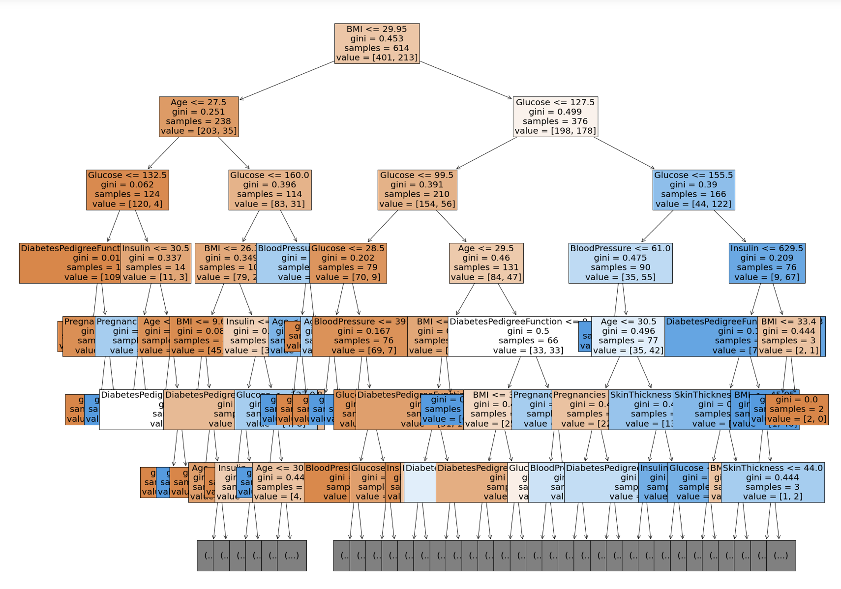

# feature 중요도 분석
model.feature_importances_
=> array([0.05537994, 0.30141185, 0.09975063, 0.03796035, 0.05168161,
       0.24775552, 0.09195419, 0.11410592])
       
# feature 중요도 시각화 
sns.barplot(x=model.feature_importances_, y=model.feature_names_in_)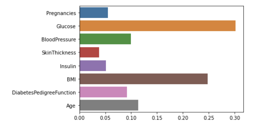

정확도(Accuracy) 측정

모델이 얼마나 잘 예측했는지 확인

from sklearn.metrics import accuracy_score

accuracy_score(y_test, y_predict)
=> 0.7792207792207793

# model의 score 로 점수 계산
model.score(X_test, y_test)
=> 0.7792207792207793