데이터 로드
df = pd.read_csv("http://bit.ly/data-diabetes-csv")
df.shape
=> (768, 9)

df.head()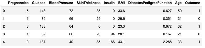
전처리
Insulin_median = df[df["Insulin"] > 0].groupby("Outcome").["Insulin"].median()
Insulin_median
=>
Outcome
0    102.5
1    169.5
Name: Insulin, dtype: float64
# 인슐린 0 값을 중앙값으로 대체
df["Insulin_fill"] = df["Insulin"]
df.loc[(df["Outcome"] == 0) & (df["Insulin_fill"] == 0), "Insulin_fill" ] = Insulin_median[0]
df.loc[(df['Outcome'] == 1) & (df['Insulin_fill'] == 0), "Insulin_fill"] = Insulin_median[1]
df[["Insulin", "Insulin_fill"]].describe()
=>
Insulin Insulin_fill
count 768.000000 768.000000
mean 79.799479 141.753906
std 115.244002 89.100847
min 0.000000 14.000000
25% 0.000000 102.500000
50% 30.500000 102.500000
75% 127.250000 169.500000
max 846.000000 846.000000학습, 예측 데이터셋
정답값이자 예측할 값
label_name = "Outcome"학습, 예측에 사용할 컬럼
feature_names = df.columns.tolist()
feature_names.remove(label_name)
feature_names.remove("Insulin")
feature_names
=> ['Pregnancies',
 'Glucose',
 'BloodPressure',
 'SkinThickness',
 'BMI',
 'DiabetesPedigreeFunction',
 'Age',
 'Insulin_fill']
문제(feature)와 답안(label) 나누기
X = df[feature_names]
y = df[label_name]
X.shape, y.shape
=> ((768, 8), (768,))
학습, 예측 데이터셋 만들기
from sklearn.model_selection import train_test_split

X_train, X_test, y_train, y_test = train_test_split(
					X, y, test_size=0.2, stratfy=y, random_state=42)

X_train.shape, X_test.shape, y_train.shape, y_test.shape
=> ((614, 8), (154, 8), (614,), (154,))

X_train.head(2)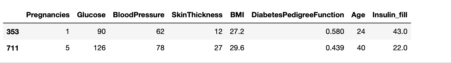
fig, axes = plt.subplots(nrows=1, ncols=2, figsize=(12, 4))
sns.countplot(x=y.train, ax=axes[0]).set_title("train")
sns.countplot(x=y.test, ax=axes[1]).set_title("test")
머신러닝 모델
from sklearn.tree import DecisionTreeClassifier

model = DecisionTreeClassifier(random_state=42)
하이퍼파라미터 튜닝
- 하이퍼파라미터 : 머신러닝 모델을 생성할 때 사용자가 직접 설정하는 값
-> 설정 정도에 따라 모델의 성능이 달라진다. - GridSearchCV() : 조합의 수 만큼 진행
-> 시도할 하이퍼파라미터를 지정하면 모든 조합에 대해 교차검증 후 가장 좋은 성능을 찾아줌 - RandomizedSearchCV() : (k-fold * n_iter) 만큼 실행
-> GridSearch와 동일한 방식이지만 모든 조합을 시도하지 않고 임의 값만 대입하여 지정된 횟수만큼 평가
GridSearchCV()
max_depth = list(range(3, 20, 2))
max_feature = [0.3, 0.5, 0.7, 0.8, 0.9]

parameters = {"max_depth" : max_depth, "max_features" : max_features}

from sklearn.model_selection import GridSearchCV
clf = GridSearchCV(model, parameters, n_job=-1, cv=5, scoring="accuracy", verbose=2)
clf.fit(X_train, y_train)

=> Fitting 5 folds for each of 45 candidates, totalling 225 fits
Out[21]:
GridSearchCV(cv=5, estimator=DecisionTreeClassifier(random_state=42), n_jobs=-1,
             param_grid={'max_depth': [3, 5, 7, 9, 11, 13, 15, 17, 19],
                         'max_features': [0.3, 0.5, 0.7, 0.8, 0.9]},
scoring='accuracy', verbose=2)clf.best_estimator_
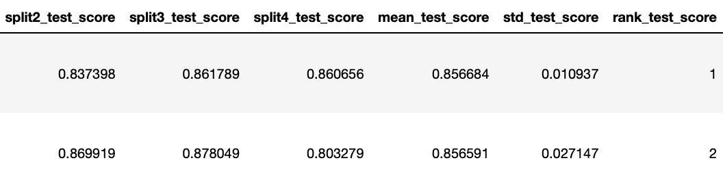
=> DecisionTreeClassifier(max_depth=9, max_features=0.5, random_state=42)pd.DataFrame(clf.cv_results_).sort_values("rank_test_score").head()
RandomizedSearchCV
# start, stop 값에 대한 랜덤 int 추출
pd.Series(np.random.randint(3, 20, 1000)).hist(figsize=(6, 2));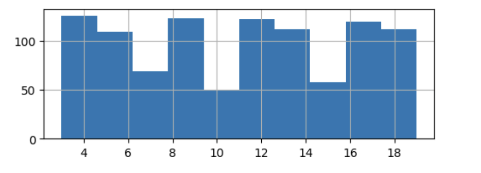
# max_features 에는 0-1 사이 값을 넣어줄 수 있도록 랜덤하게 생성
Pd.Series(np.random.uniform(0.5, 1, 1000)).hist(figsize=(6, 2));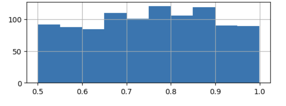
from sklearn.model_selection import RandomizedSearchCV
# RandomizedSearchCV : cv(k-fold) * n_iter 수 만큼 실행
param_distributions = {"max_depth" : np.random.randint(3, 25, 10),
                       "max_features" : np.random.uniform(0.55, 1, 10)}

clfr = RandomizedSearchCV(model,
                   param_distributions=param_distributions,
                   n_iter=10,
                   cv=5,
                   scoring="accuracy",
                   n_jobs=-1,
                   random_state=42, verbose=3)
clfr.fit(X_train, y_train)
=>
Fitting 5 folds for each of 10 candidates, totalling 50 fits
Out[26]:
RandomizedSearchCV(cv=5, estimator=DecisionTreeClassifier(random_state=42),
                   n_jobs=-1,
                   param_distributions={'max_depth': array([24, 17, 14, 17, 23, 21, 20, 13, 15, 16]),
                                        'max_features': array([0.92284167, 0.71087365, 0.98375356, 0.90413657, 0.95225597,
       0.73280807, 0.76763317, 0.88356566, 0.94046386, 0.81585744])},
random_state=42, scoring='accuracy', verbose=3)clfr.best_estimator_
=> DecisionTreeClassifier(max_depth=23, max_features=0.7328080663623351,
random_state=42)
clfr.best_params_
=> {'max_features': 0.7328080663623351, 'max_depth': 23}Best Estimator
# 데이터를 머신러닝 모델로 학습(fit)
best_model = clfr.best_estimator_
best_model.fit(X_train, y_train)

=> DecisionTreeClassifier(max_depth=23, max_features=0.7328080663623351,
                       random_state=42)

# 데이터를 머신러닝 모델로 예측(predict)
y_predict = best_model.predict(X_test)

# 정확도 확인
(y_test == y_predict).mean()
=> 0.8441558441558441
모델 평가 feature importances
# feature_importances_ 를 통한 피처 중요도 추출
best_model.feature_importances_
=> array([0.03922289, 0.08736366, 0.0330258 , 0.11433261, 0.07114157,
       0.04905032, 0.08087602, 0.52498713])

# 피처 중요도 시각화
sns.barplot(x=best_model.feature_importances_, y=best_model.feature_names_in_)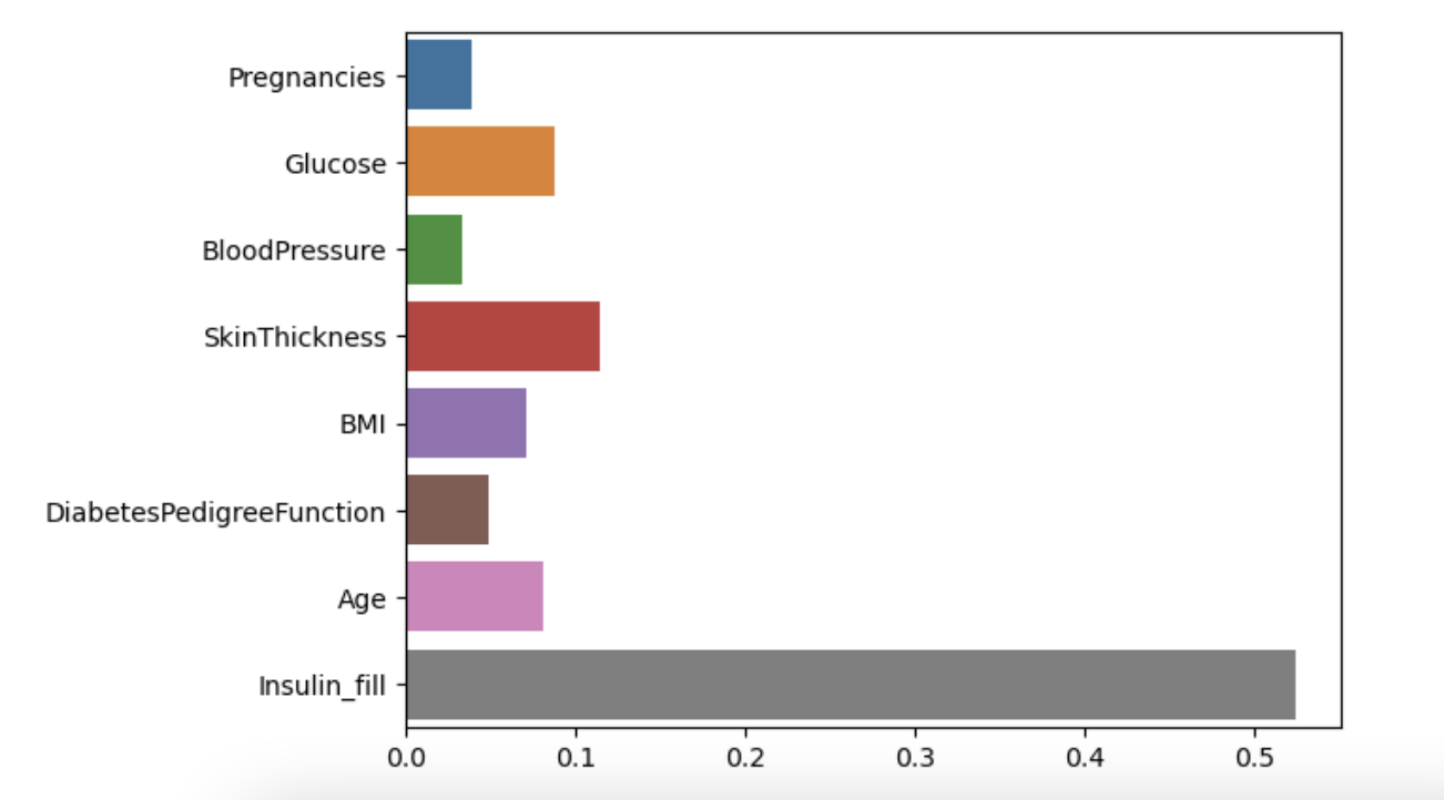
Accuracy 측정
from sklearn.metrics import accuracy_score

accuracy_score(y_test, y_predict)
=> 0.8441558441558441

from sklearn.metrics import classification_report

print(classification_report(y_test, y_predict))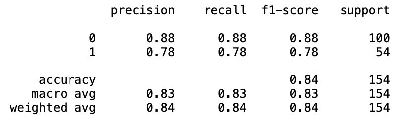

Ⓓ🅰️🅣🄰 ♡♥︎