Pytorch를 간단히 다루어본 적이 있는데, 앞으로의 연구에 익숙하게 활용하기 위해 Pytorch 내용을 정리해보려 한다.

대부분의 내용은 유튜브의 '모두를 위한 딥러닝 시즌2'를 참고하였다.

기본적인 딥러닝 내용은 어느 정도 알고 있다고 가정하고, PyTorch 실습 내용 위주로 정리해두었다.

간단한 설명이 포함된 실습 자료는 다음 Github를 참조하자.

1. Basic Approach to Train Deep Neural Network

딥러닝 모델을 구축할 때 기본적인 절차를 살펴보자.

1. Neural Network Architecture 설계
   • 목적에 맞는 딥러닝 모델을 설계한다.
2. 학습을 시킨 후, 모델이 ovefitting되지는 않았는지 확인한다. (Training loss는 줄어들지만 Validation Loss는 오히려 커지는 경우)
   • overfitting되지 않았다면 모델의 사이즈를 키우고 (깊거나 넓게)
   • overfitting되었다면 dropout, batch-normalization 등의 방법을 추가하여 overfitting을 방지해준다.
3. Step '2.'를 반복한다.

Implementation

실습을 통해 딥러닝 모델을 만드는 과정을 살펴보자.

1) Import

먼저, 필요한 라이브러리를 import한다.

import torch
import torch.nn as nn
import torch.nn.functional as F
import torch.optim as optim

# For reproducibility
torch.manual_seed(1)

2) Training and Test Dataset

다음으로, training set과 test set을 나누어준다.

# training set
x_train = torch.FloatTensor([[1, 2, 1],
                             [1, 3, 2],
                             [1, 3, 4],
                             [1, 5, 5],
                             [1, 7, 5],
                             [1, 2, 5],
                             [1, 6, 6],
                             [1, 7, 7]
                            ]) # (8, 3)
y_train = torch.LongTensor([2, 2, 2, 1, 1, 1, 0, 0]) # (8, )

# test set
x_test = torch.FloatTensor([[2, 1, 1], [3, 1, 2], [3, 3, 4]]) # (3, 3)
y_test = torch.LongTensor([2, 2, 2]) # (3, )

여기서 분류할 class 개수는 3개이고, train sample은 8개, test sample은 3개임을 알 수 있다.

3) Model

다음으로 softmax classification 모델을 생성해보자. 자세한 방법은 이전 포스팅에 설명되어있다.

class SoftmaxClassifierModel(nn.Module):
    def __init__(self):
        super().__init__()
        self.linear = nn.Linear(3, 3)
    def forward(self, x):
        return self.linear(x)

model = SoftmaxClassifierModel()

# Optimizer 설정
optimizer = optim.SGD(model.parameters(), lr=0.1)

4) Training

이어서 다음과 같이 학습을 진행한다.

def train(model, optimizer, x_train, y_train):
    nb_epochs = 20
    for epoch in range(nb_epochs):
        # H(x) 계산
        prediction = model(x_train)
        # cost 계산
        cost = F.cross_entropy(prediction, y_train)
        # cost로 H(x) 개선
        optimizer.zero_grad()
        cost.backward()
        optimizer.step()
        
        print('Epoch {:4d} / {} Cost: {:.6f}'.format(
            epoch, nb_epochs, cost.item()
        ))

5) Test (Validation)

Training 후에는 Overfitting 여부를 판단하기 위해 test dataset에 대해 test dataset에 대해 test를 진행한다.

여기서는 validation과 같은 용어를 사용하지만, 엄밀히 말하자면 validation은 학습과정 내에서 모델의 하이퍼파라미터를 조정해주기 위한 평가 과정이고, test는 학습이 모두 종료된 이후, generalization이 잘 되었는지 평가하는 과정이다.

즉, validation dataset은 training dataset의 일부를 사용하는 경우가 많으며, test dataset은 unseen data(본 적 없는 데이터)를 사용한다.

def test(model, optimizer, x_test, y_test):
    prediction = model(x_test)
    predicted_classes = prediction.max(1)[1]
    correct_count = (predicted_classes == y_test).sum().item()
    cost = F.cross_entropy(prediction, y_test)
    
    print('Accuracy: {}% Cost: {:.6f}'.format(
        correct_count / len(y_test) * 100, cost.item()
    ))

모델에 test 입력을 주고 마찬가지로 cross_entropy를 사용하여 예측된 클래스와 실제 클래스가 같은지 확인해준다.

6) Run

간단히 위에서 정의한 함수를 호출하여 train과 test를 진행한다.

[train]

train(model, optimizer, x_train, y_train)

[test]

test(model, optimizer, x_test, y_test)

Train과 test 결과는 다음과 같다.

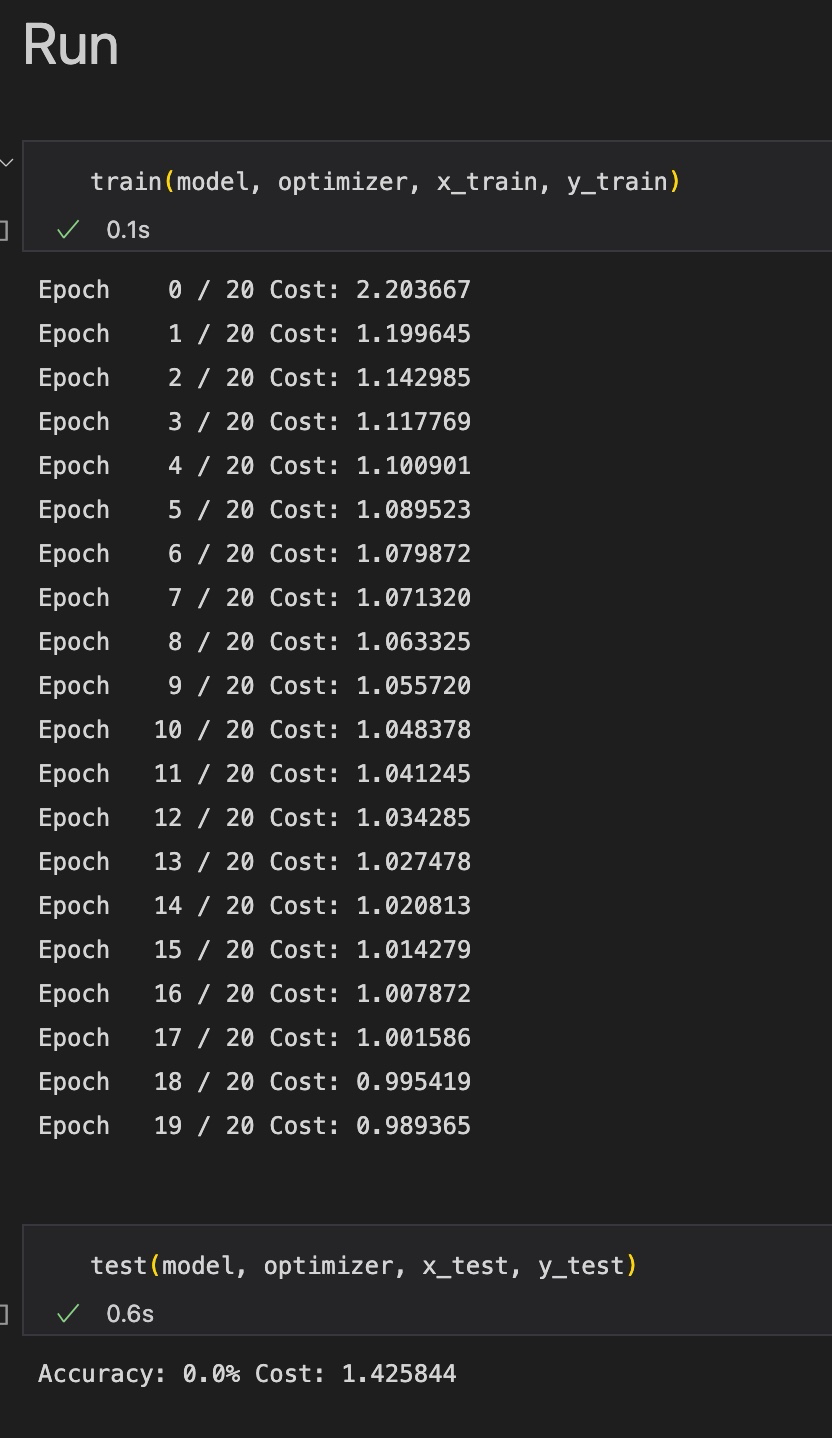
결과에서 train data에 대한 cost는 계속 떨어지지만, test data에 대한 cost는 1.4로 매우 높다. 따라서 overfitting이 발생했음을 알 수 있다.

7) Generalization 성능을 높이는 방법들

overfitting을 완화하기 위해서는 Regularization을 적용하거나, 여러가지 hyperaparmeter를 조정해주거나, 데이터를 정제해주는 등의 방법이 있다.

우리가 이제까지 크게 신경쓰지 않고 써왔던 'learning rate'가 바로 대표적인 hyperparameter의 예이다.

값이 너무 크면 cost 값이 줄지 않고 발산해버리고, 너무 작으면 cost가 너무 늦게 줄어든다.

코드에서 'optimizer'를 정의할 때 lr의 값을 조정하면 된다.

데이터를 사전에 정제해주는 작업인 Data Preprocessing(전처리) 과정의 대표적인 예시는 'Standardization(표준화, normalization)'이 있다. 이는 다음과 같은 수식으로 진행한다.

$x'_{j} = \frac{x_j - \mu_j}{\sigma_j}$

여기서 $\sigma$는 데이터의 standard deviation, $\mu$는 데이터의 평균값이다.

코드로 다음과 같이 구현할 수 있다.

mu = x_train.mean(dim=0)
sigma = x_train.std(dim=0)
normalized_x_train = (x_train - mu) / sigma
print(normalized_x_train)

print된 값들은 표준정규분포를 따른다.

2. MNIST

딥러닝 계의 'Hello World!'인 MNIST 데이터셋에 대한 딥러닝 모델을 간단히 만들어보자.

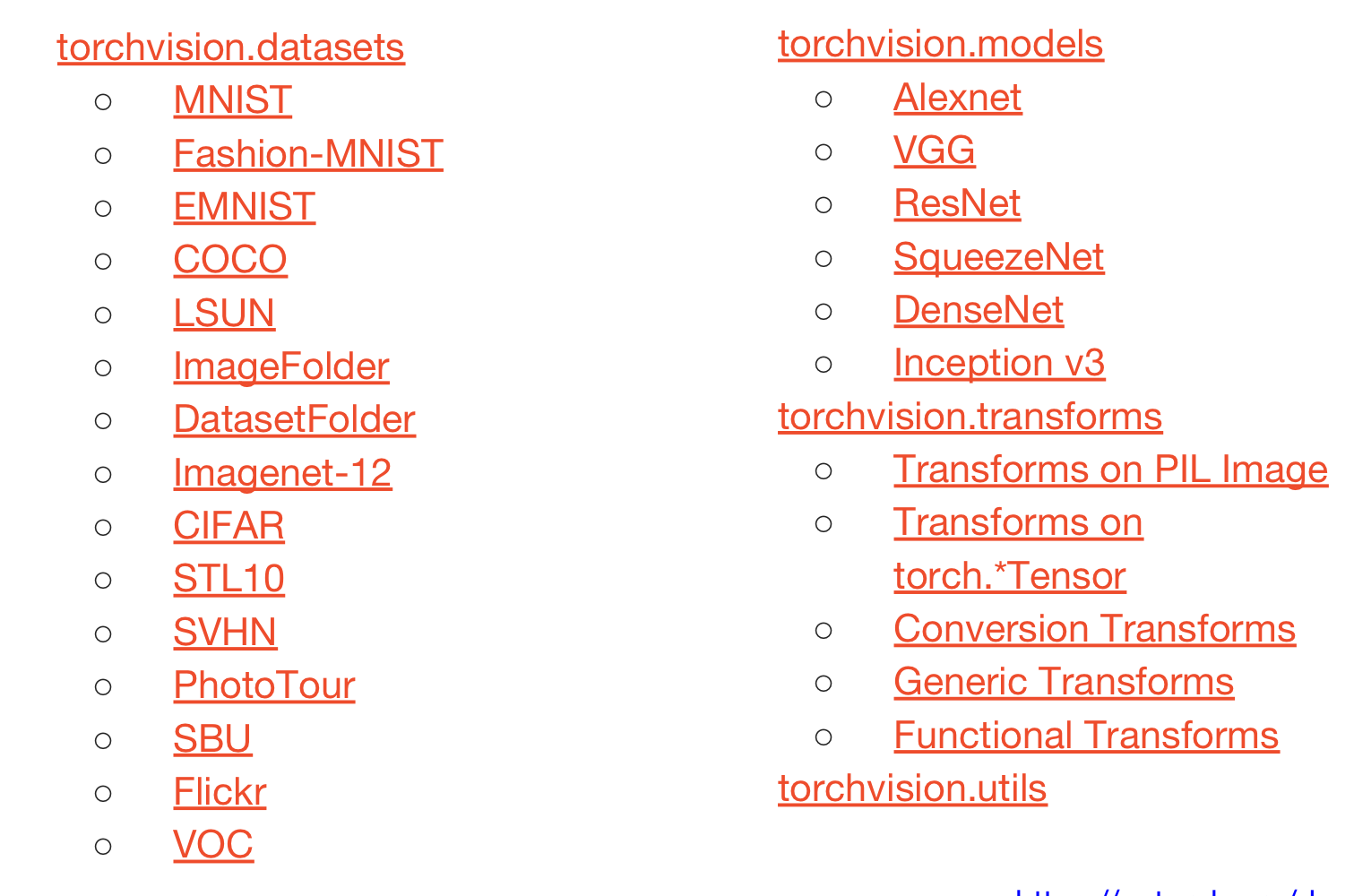
먼저, 'torchvision'이라는 패키지에 대해 알아둘 필요가 있다.

torchvision 패키지는 PyTorch에서 제공하는 유명한 데이터셋, 모델, transforms 등을 포함하는 라이브러리이다.

1) Reading Data

torchvision에 포함된 데이터셋을 불러오는 과정은 다음과 같다.

import torch
import torch.nn as nn
import torch.nn.functional as F
import torch.optim as optim
import torchvision.datasets as dsets
import torchvision.transforms as transforms
import matplotlib.pyplot as plt
import random

mnist_train = dsets.MNIST(root="MNIST_data/", train=True, transform=transforms.ToTensor(), download=True)
mnist_test = dsets.MNIST(root="MNIST_data/", train=False, transform=transforms.ToTensor(), download=True)

# parameters
training_epochs = 15
batch_size = 100

data_loader = torch.utils.data.DataLoader(dataset=mnist_train, batch_size=batch_size, shuffle=True, drop_last=True)

MNIST 함수의 인자는 각각 다음을 의미한다.

• root : MNIST 데이터가 어느 경로에 있는지를 나타낸다.
• train : train data인지(true), test data인지(false)를 나타낸다.
• transform : MNIST 이미지를 불러올 때 어떤 transform을 적용할지를 나타낸다.
  • 일반적으로 PyTorch에서 받아들이는 이미지는 0에서 1 사이의 값을 가지며, 순서는 Channel-Height-Weight이다. 하지만 이미지는 0-255의 값을 가지며, 순서가 Height-Weight-Channel이다.
  • 원래 이미지의 형태를 PyTorch에서 받아들일 수 있도록 바꾸어주는 과정이 'transforms.ToTensor()'함수이다.
• download에 True를 부여하면 root 경로에 MNIST 데이터가 존재하지 않으면 다운을 받는다는 의미를 갖는다.

DataLoader 함수 인자는 다음과 같은 의미를 갖는다.

• DataLoader : 어떤 데이터를 불러올 것인지를 의미한다.
• batch_size : train 이미지를 몇 개씩 잘라서 갖고올 것인지를 의미한다.
• shuffle : 순서를 섞을지 여부를 나타낸다.(보통 True)
• drop_last : batch_size만큼 잘라서 사용하고 남은 데이터를 버릴지를 나타낸다. (True 시 버림)

epoch 내에서 iterable variable인 data_loader에 따라 'view'함수를 사용하여 28 * 28 사이즈를 (, 784)의 사이즈로 바꾼다.

Terminology : Epoch/Batch size/Iteration

Neural Network에서 자주 사용하는 용어를 정리해보자.

• epoch : 모든 training samples에 대해 한 번의 forward pass와 backward pass를 진행할 때, 1 epoch이라 한다.
• batch size : 학습 시간을 줄이고, 한정적인 메모리 용량을 효율적으로 사용하도록 training sample 전체를 'batch_size'만큼 잘라 forward/backward pass를 진행한다. 예를 들어, 총 60000장의 이미지가 있고, 100장씩 나누어 학습을 진행한다면 batch size는 600이 된다.
  • batch size가 커질수록 필요한 메모리가 커진다.
• iterations : batch를 학습에 몇 번 사용했는가를 나타낸다. 위의 예시에서 1epoch을 돌기 위해서는 100 iteration이 필요하다.

$\text{1 epoch} = \text{batch size} × \text{iterations}$

2) Training with Softmax Classifier

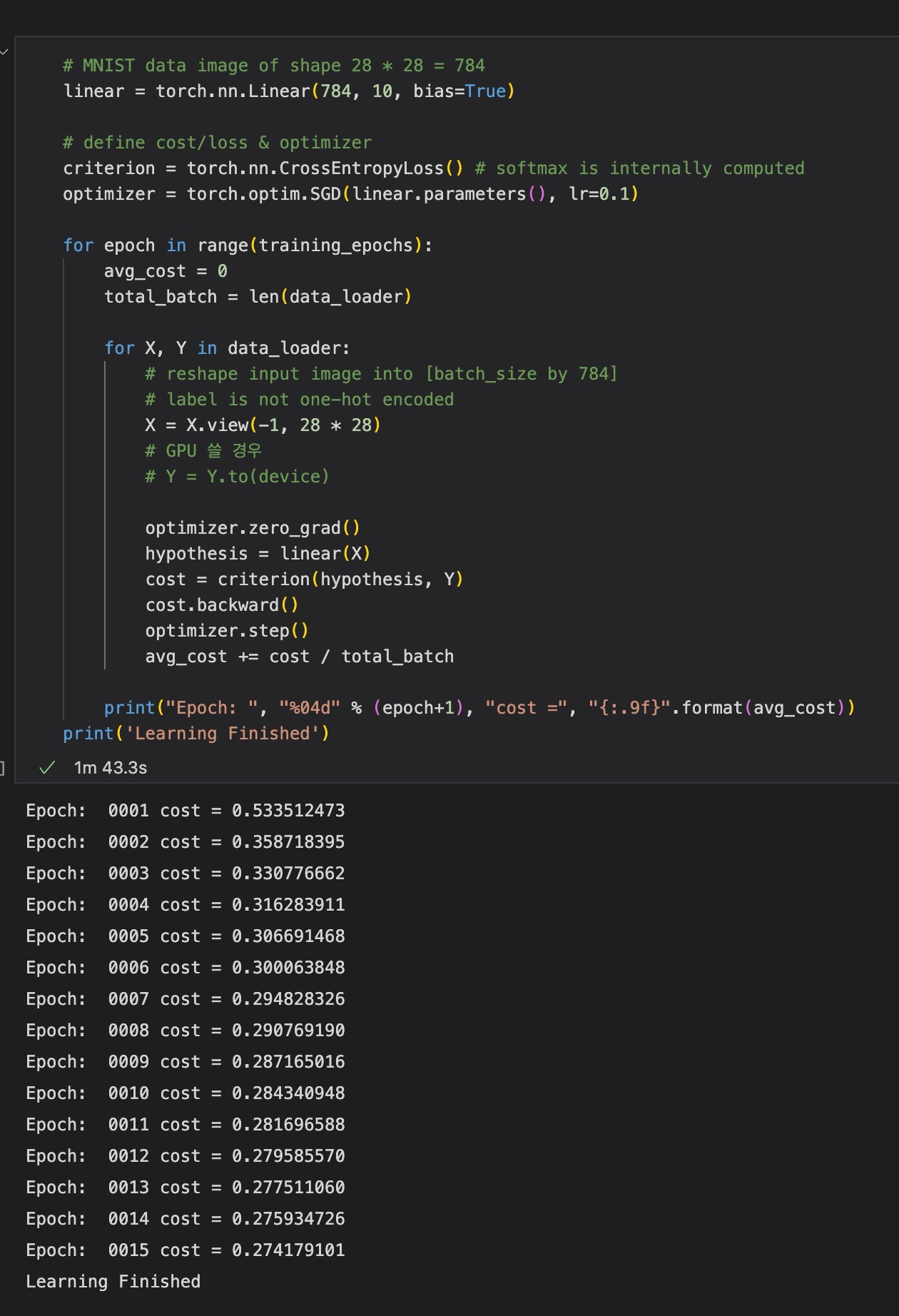
# MNIST data image of shape 28 * 28 = 784
linear = torch.nn.Linear(784, 10, bias=True)

# define cost/loss & optimizer
criterion = torch.nn.CrossEntropyLoss() # softmax is internally computed
optimizer = torch.optim.SGD(linear.parameters(), lr=0.1)

for epoch in range(training_epochs):
    avg_cost = 0
    total_batch = len(data_loader)
    
    for X, Y in data_loader:
    	# reshape input image into [batch_size by 784]
        # label is not one-hot encoded
        X = X.view(-1, 28 * 28)
        # GPU 쓸 경우
        # Y = Y.to(device)
        
        optimizer.zero_grad()
        hypothesis = linear(X)
        cost = criterion(hypothesis, Y)
        cost.backward()
        optimizer.step()
        avg_cost += cost / total_batch
    
    print("Epoch: ", "%04d" % (epoch+1), "cost =", "{:.9f}".format(avg_cost))
print('Learning Finished')

결과는 아래와 같다.

3) Test & Visualization

이제 test dataset을 통해 모델이 예측을 잘 해내는지 알아보자.

# Test the model using test sets
with torch.no_grad():
    X_test = mnist_test.test_data.view(-1, 28 * 28).float()
    Y_test = mnist_test.test_labels
    
    prediction = linear(X_test)
    correct_prediction = torch.argmax(prediction, 1) == Y_test
    accuracy = correct_prediction.float().mean()
    print('Accuracy: ', accuracy.item())
    
    # Get one and predict
    r = random.randint(0, len(mnist_test) - 1)
    X_single_data = mnist_test.test_data[r:r + 1].view(-1, 28 * 28).float()
    Y_single_data = mnist_test.test_labels[r:r + 1]
    
    print('Label: ', Y_single_data.item())
    single_prediction = linear(X_single_data)
    print('Prediction: ', torch.argmax(single_prediction, 1).item())
    
    plt.imshow(mnist_test.test_data[r:r + 1].view(28, 28), cmap='Greys', interpolation='nearest')
    plt.show()

여기서, torch.no_grad()란, gradient를 계산하지 않겠다는 의미이다. test 시에는 gradient를 계산하지 않아야 하므로, 위와 같이 with 구문을 통해 실수를 방지할 수 있다.

결과는 다음과 같다.

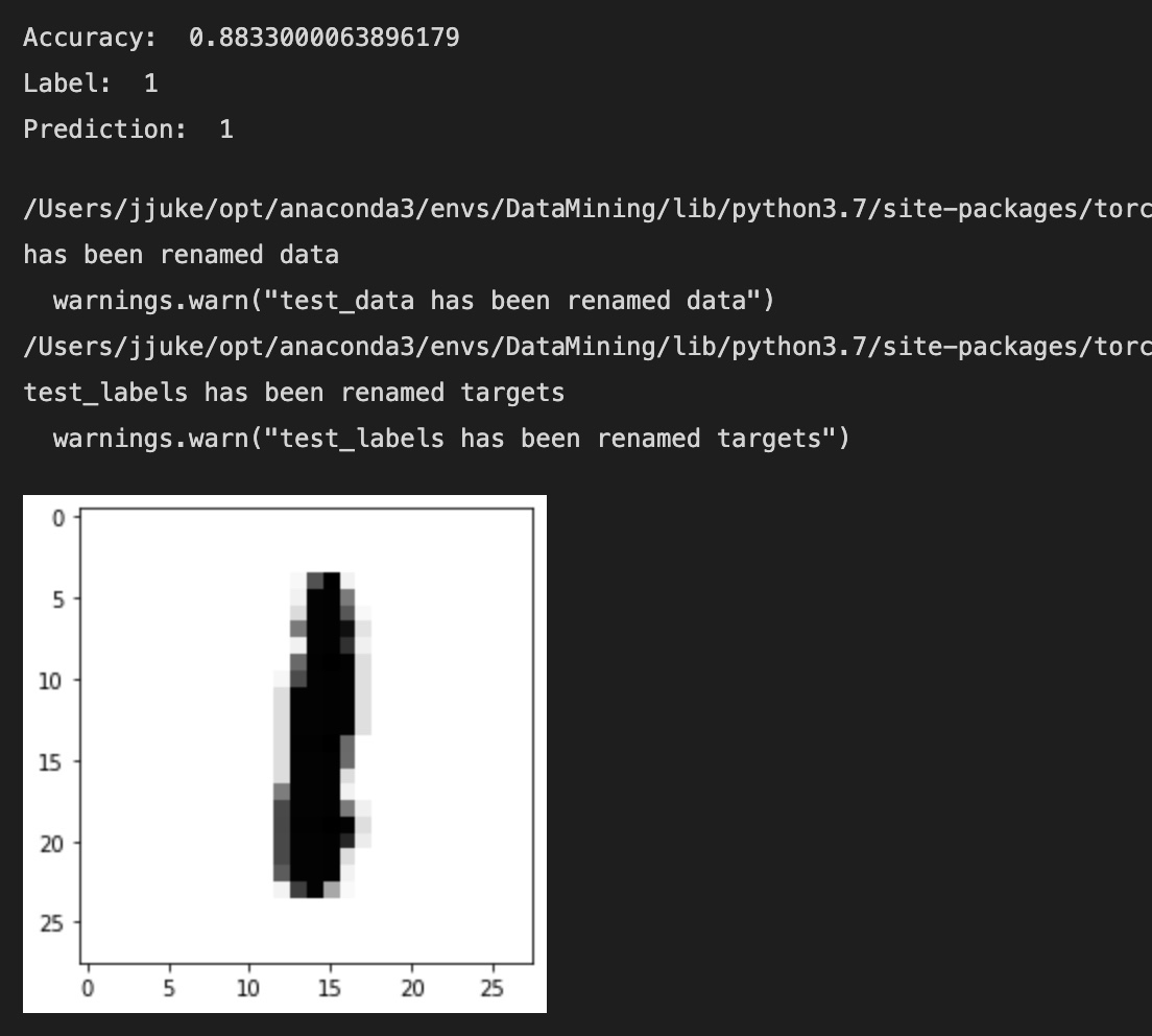
모델이 실험 데이터에 대해서 약 88%의 정확도를 갖는 것을 확인할 수 있다.