Day 1

쉬는 날이지만 이제는 쉬는 날도 맘 편히 쉴 수 없을 것 같아서 강의를 듣기로 했다... 이제는 이런 날이 일상이 되겠지..?

강의 듣기 - Computer Vision (1)

Computer Vision 이란??

Why is visual perception important?

• About 75% of information comes through our eyes.
• More than 50% of the brain is devoted to processing visual info.
• Computer vision은 Computer Graphic의 역 연산이라고 생각할 수 있음.

What is Computer Vision?

• Machine Learning : Input -> Feature Extraction -> Classification -> Output
• Deep Learning : Input -> Feature Extraction + Classification -> Output.
  • 더 쉽고, 더 간단하게, 더 성능이 좋게 할 수 있음.

Image Classification

• Classifier : A mapping f(.) that maps an image to a category level
  • How to? : What if we could memorize all the data in the world? -> All the classification problems could be solved by k-NN algorithm.
    But, Time complexity and Memory complexity goes to infinity. And it is hard to define how to compare similarity of the pictures.
  • How to? : Compress all the data we have into the neural network
  • CNN
    - Convolution Neural Networks are locally connected neural networks with sliding window. -> Local feature learning, Parameter sharing, Less parameters.
    • CNN is used as a backbone of many CV tasks. Extract features of the image or video.

CNN architectures for image classification

• Brief History : AlexNet -> VGGNet -> GoogLeNet -> ResNet -> ...
  • AlexNet
    - Overall Architecture : 5 Conv Layers, 3 FC Layers.
    • Deprecated components 1. Local Response Normalization (LRN)
      • Lateral inhibition : the capacity of an excited neuron to subdue its neighbors
      • LRN normalizes around the local neighborhood of the excited neuron
      • Excited neuron becomes even more sensitive as compared to its neighbors
      • 명암을 더 명확하게
    • Deprecated components 2. 11 * 11 conv filter
      • Larger size filters are used to cover a wider range of the input image.
  • VGGNet
    • Deeper architecture (16 and 19 layers)
    • Simpler architecture (No LRN, only 3*3 conv filter, 2*2 max pool)
    • Better performance
    • Better generalization
    • Key design choices
      • Using many 3*3 conv layers instead of a small number of larger conv filters.
        • Keeping receptive field sizes large enough
        • Deeper with more non-linearities
        • Fewer parameters

Day 2

깃헙 특강 (1)

강의 듣기 - Computer Vision (1)

Annotation data efficient learning

Learning representation of dataset

• Dataset is almost always biased
• Images taken by camera (training data) $\neq$ real data
• i.e. The training dataset contains only fractional part of real data.
• Suppose a training dataset has only bright images
  • During test time, if a dark image is fed as input, the trained model may be confused.
  • Problem : Datasets do not fully represent real data distribution!
• Sol : Augmenting data!
  • Brightness
  • Rotation
  • Crop
  • Affine transformation (shear)
  • And so on...

Modern Augmentation Techniques

• CutMix
  • Mixing both images and labels
• RandAugment
  • Many augmentation methods exist. Hard to find the best augmentations to apply
  • Automatically finding the best sequence of augmentations to apply
  • Random sample, apply and evaluate augmentations.
  • Two params : Which augmentation to apply, Magnitude of augemntation to apply (how much augment)

Leveraging pre-trained information

Transfer Learning

• The high-quality dataset is expensive and hard to obtain.
  • Supervised learning requires a very large-scale dataset for training
  • Annotating data is very expensive, and its quality is not ensured
  • Transfer Learning : A practical training method with a small dataset
• We can easily adapt to a new task by leveraging pre-trained knowledge(feature)!
• Method1
  • Freeze weights of the Conv layer, 마지막 fc layer만 교체하여 학습
• Method2
  • Conv layer는 low learning rate로 학습, 마지막 fc layer 교체하고 high learning late로 학습
• Method3 : Knowledge Distillation
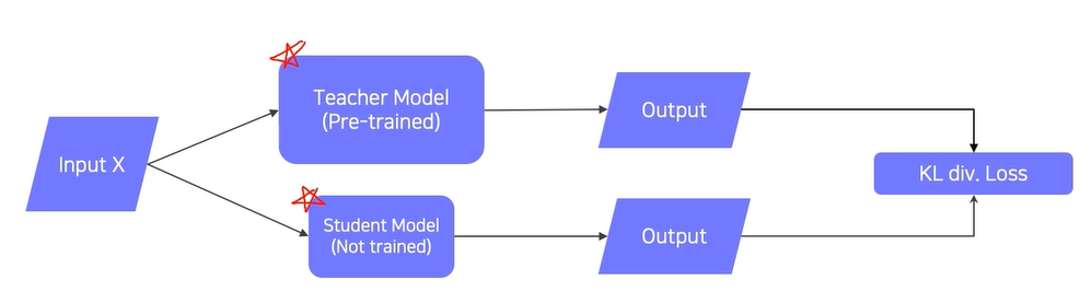
  • Distillate knowledge of a trained model into another smaller model
  • Used for model compression (Mimicking what a larger model knows)
  • Also, used for pseudo-labelling (Generating pseudo-labels for an unlabeled dataset), 즉, 큰 모델에서 나온 결과를 unlabeled data의 label로 활용하여 학습.
  • When train with unlabeld data (=unsupervised learning)
    • 
  • When train with both labeled and unlabled data
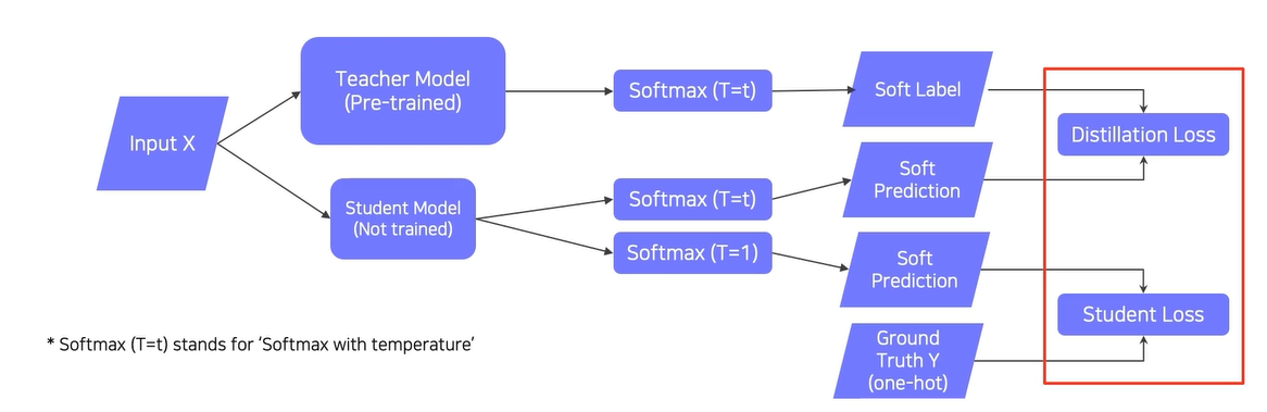
    • Student loss : When labeled data is available, can leverage labeled data for training. (Cross Entropy).
      Learn the 'right answer'
    • Distillation loss to 'predict similar outputs with the teacher model' (KL divergence).
      Learn what teacher network knows by mimicking
    • Soft Prediction : 실수값으로써 label의 확률을 나타내는 것. 대표적으로는 softmax의 output.
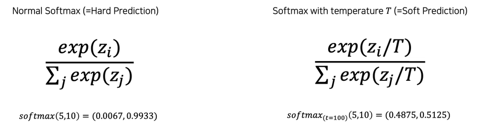
    • Softmax with Temperature(T)
      • Softmax with temperature : controls difference in output between small & large input values
      • A large T smoothens large input value differences
      • Useful to synchronize the student and teacher models' outputs
      • 
    • Semantic information is not considered in distillation. "Teacher model의 요소 하나하나가 중요하다기 보다는 Teacher model이 어떻게 생각을 하는지를 배우는 것이다." 라고 이해하자.
    • 

Leveragning unlabeled dataset for training

Semi-supervised learning

• Unsupervised (No label) + Fully Supervised (fully labeled)
• Pseudo-labeling unlabeled data using a pre-trained model, then use for training
  

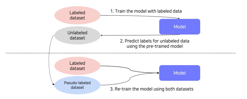
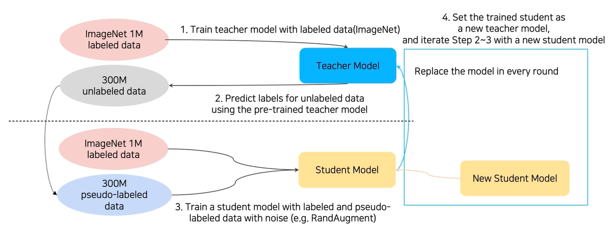
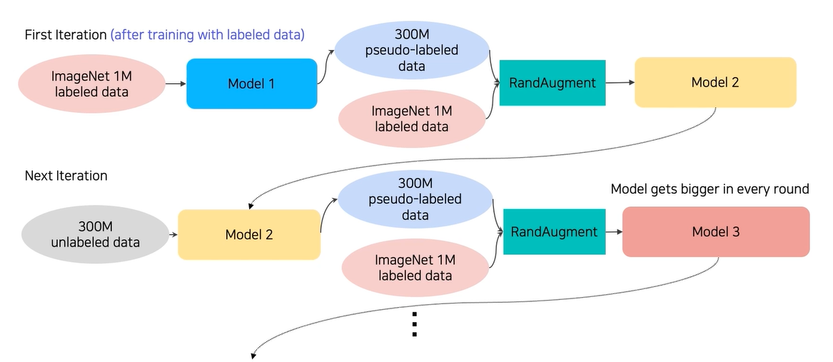
Self-training - Noisy Student Learning

• Augmentation + Teacher-Student Networks + semi-supervised learning
• 
• 

Problems with deeper layers

Going deeper with convolutions

• The neural network is getting deeper and wider
• Deeper networks learn more powerful features, because of Larger receptive fields and More capacity and non-linearity
• Deeper networks are harder to optimize
  • Gradient vanishing / exploiding
  • Computationally complex
  • Degradation Problem

GoogLeNet

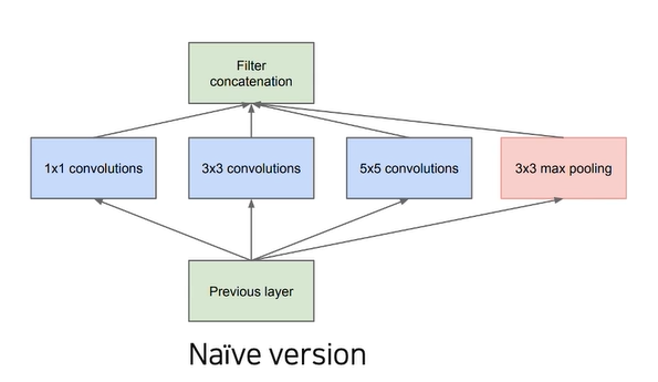
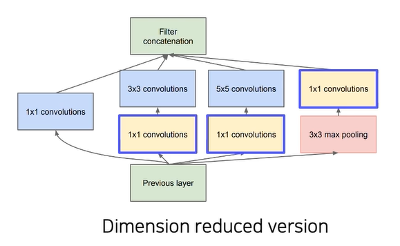
• Inception module
  • Apply multiple filter operations an input activationfrom the previous layer
    • 1*1, 3*3, 5*5 convolution filters
    • 3*3 pooling operation
  • Concatenate all filter outputs together along the channel axis
    
  • Problem : The increased network size increases the use of computational resources.
  • Sol : Use 1*1 convolutions and reduce the number of channels (Bottleneck layers).
    
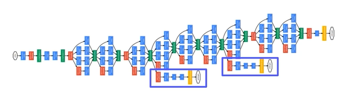
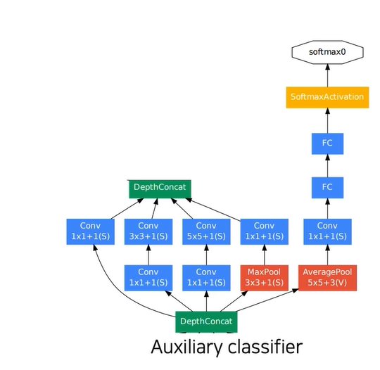
• Auxiliary classifier
  • The vanishing gradient problem is dealt with by the auxiliary classifier
  • Injecting additional gradients into lower layers
    
  • Used only during training, removed at testing time
    

ResNet

• Building Ultra-deeper than any other networks
• But building a very deep architecture is hard.
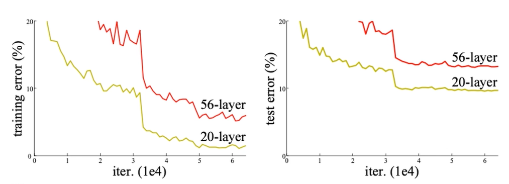
  • Degradation Problem
    • As the network depth increases, accuracy gets saturated -> degrade rapidly
    • 
    • Above picture shows that this is not caused by overfitting. The problem is optimization! (오버피팅이라면 training error는 56 layer가 더 낮지만 test error는 56 layer가 더 높아야 하는데, train, test 둘다 56 layer가 더 높은 error를 기록함.)
• Hypothesis
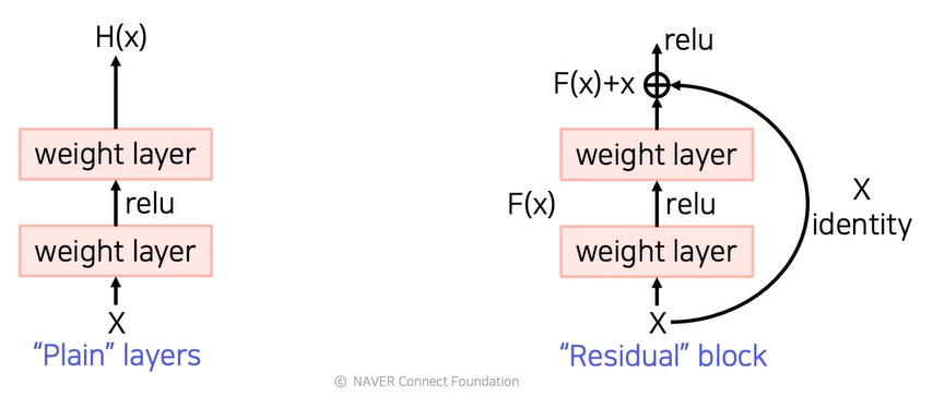
  • Plain Layer : As the layer get deeper, it is hard to learn good $H(x)$ directly
  • Residual Block : Instead, we learn residual
    • Target function : $H(x)=F(x)+x$
    • Residual function : $F(x)=H(x)-x$
      
• Solution : Shortcut connection (=Skip connection)
  • Use layers to fit a residual mapping instead of directly fitting a desired underlying mapping
  • The vanishing gradient problem is solved by shortcut connection
  • Don't just stack layers up, instead use shortcut connection!
• Why it works better?
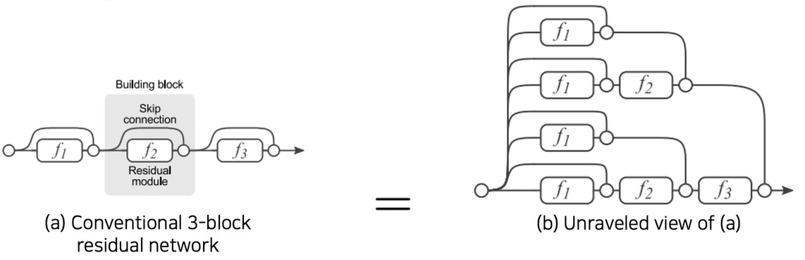
  • During training, gradients are mainly from relatively shorter paths
  • Residual networks have $\mathcal{O}(2^n)$ implicit paths connecting input and output, and adding a block doubles the number of paths.
    

Beyond ResNet - DenseNet

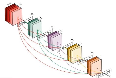
• In ResNet, we added the input and the output of the layer element-wisely
• In the Dense Blocks, every output of each layer is concatenated along the channel axis.
  • Alleviate vanishing gradient problem
  • Strengthen feature propagation
  • Encourage the reuse of features
    

Beyond ResNet - SENet (Squeeze and Excitation)

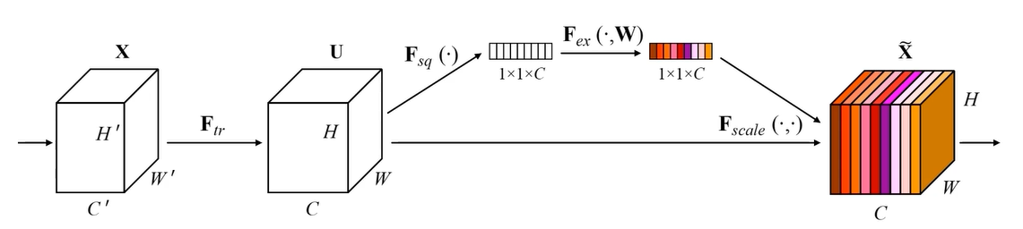
• Attention across channels
• Recalibrates channel-wise responses by modeling interdependencies between channels
• Squeeze and excitation operations
  • Squeeze : capturing distributions of channel-wise responses by global average pooling
  • Excitation : gating channels by channel-wise attention weights obtained by a FC layer
    

Beyond ResNet - EfficientNet

• Building deep, wide, and high resolution networks in an efficient way.

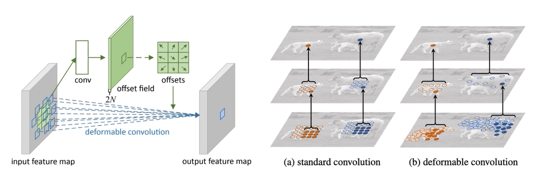
Beyond ResNet - Deformable convolution

• 2D spatial offset prediction for irregular convolution
• Irregular grid sampling with 2D spatial offsets
• Implemented by standard CNN and grid sampling with 2D offsets
  

Day 4

강의 듣기 - Semantic Segmentation, Object Detection

Semantic segmentation

What is Semantic segmentation

• Classify each pixel of an image into a category
• Don't care about instances. Only care about semantic category. 사람의 class에 대해서 분류하지 그 안에서 다른 사람들끼리 구분하진 못함. 다른 사람들까지 구분하려면 instance segmentation

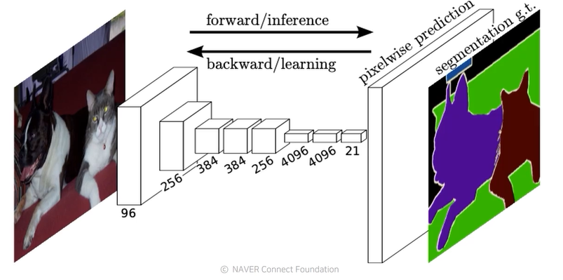
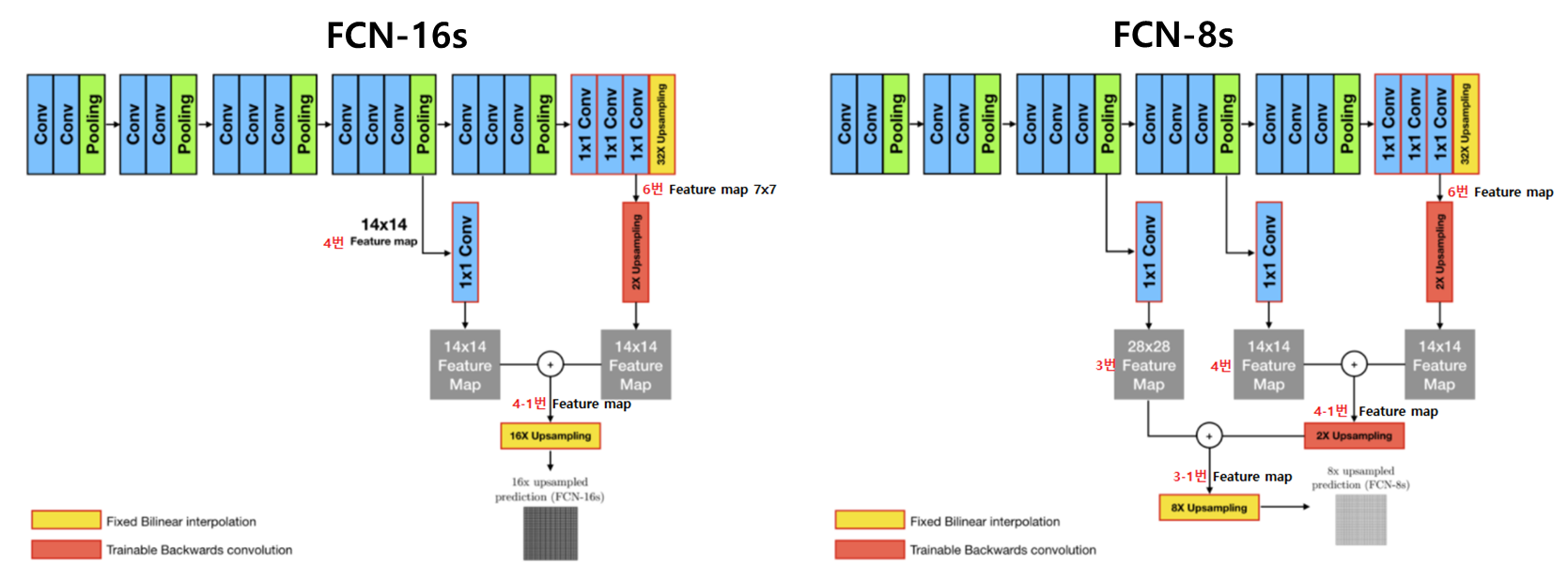
Fully Convolutional Networks

• The first end-to-end architecture for semantic segmentation
• Take an image of an arbitrary size as input, and output a segmentation map of the corresponding size to the input
  
• Fully Connected vs Fully Convolution
  • Fully Connected : Output a fixed dimensional vector and discard spatial coordinates. It classifies a single feature vector. 공간 정보를 고려하지 않음.
  • Fully Convolutional : Output a classification map which has spatial coordinates. It classifies every feature vector of the convolutional feature map. 공간 정보를 고려함.
• Limitation : Predicted score map is in a very low-resolution.
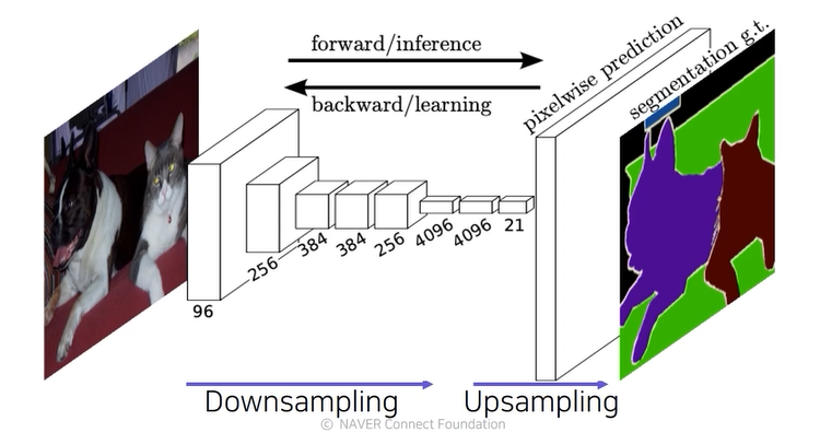
• Solution : Enlarge the score map by upsampling!

Upsampling

• The size of the input image is reduced to a smaller feature map.
• Upsample to the size of input image.
  
• Methods
  • Unpooling
  • Transposed convolution
  • Upsample and convolution
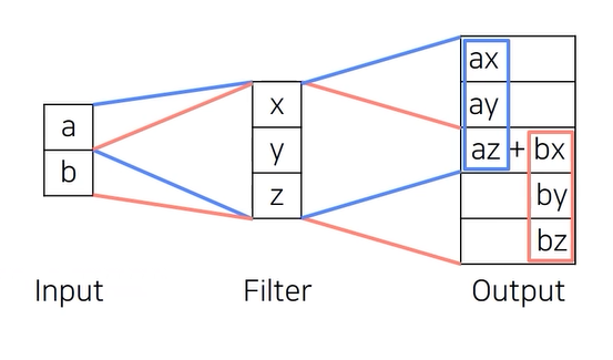
• Transposed Convolution
  • It works by swapping the forward and backward passes of convolution.
  • Problems : az+bx가 계속 중첩되는데 괜찮은가? Checkerboard artifacts due to uneven overlaps. -> Tuning으로 조절..
    
• Upsampling and convolution
  • Avoid overlap issues in transposed convolution
  • Decompose into spatial upsampling and feature convolution
    - {Nearest Neighbor, Bilinear} interpolation follwed by convolution
    

FCN with upsampling

• Adding skip connections for enlarging the score map
  • 초기의 activation map들은 receptive field size가 작기 때문에 국지적이고 detail을 보고 작은 차이에도 민감함.
  • 마지막 단의 activation map들은 해상도는 낮지만 큰 receptive field를 갖기 때문에 전역적이고 의미론적인 정보들을 포함함.
  • 마지막 단의 activation map들을 upsampling 하여 해상도를 올리고, 중간 층의 activation map을 upsampling한다. 그리고 concat 하여 사용한다.
    
• Features of FCN
  • Faster : The end-to-end architecture that does not depend on other hand-crafted components.
  • Accurate : Feature representation and classifiers are jointly optimized.

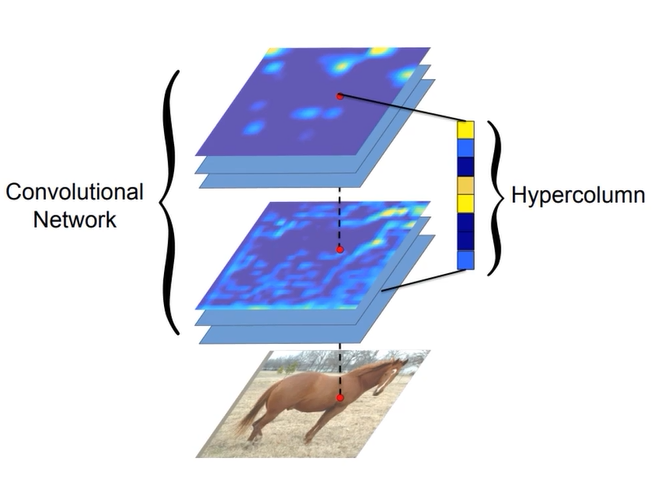
Hypercolumns for object segmentation

• CNN layers typically use the output of the last layer as feature representation
  • Too coarse spatially
• Hypercolumn at a pixel is a stacked vector of all CNN units on that pixel
  • Fine localized information is extracted from earlier layers.
  • Coarse semantic information is extracted from latter layers.
    
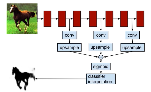
• Overall Architecture
  • Very similar to FCN
  • Difference : Apply to each bounding box
    

U-Net

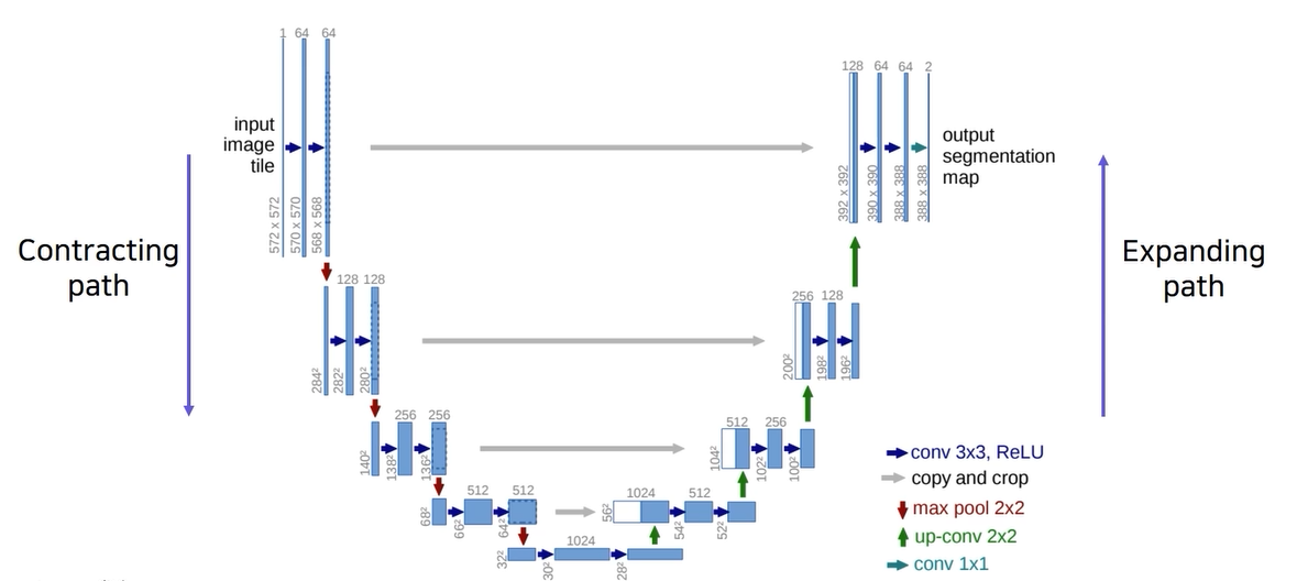
• Built upon 'fully convolutional networks'
  • Share the same FCN property
• Predict a dense map by concatenating feature maps from contracting path
  • Similar to skip connections in FCN
• Yield more precise segmentations
• Architecture
  
  • Contracting Path : Halve the size of the feature map
    • Repeatedly applying 3*3 convolutions
    • Doubling the number of feature channels
    • Being used to capture holistic context
    • Halve the size of the feature map
    • Double the channel of the feature map
  • Expanding Path
    • Repeatedly applying 2*2 convolutions
    • Halving the number of feature channels
    • Concatenating the corresponding feature maps from the contracting path.
    • Double the size of the feature map
    • Halve the channel of the feature map
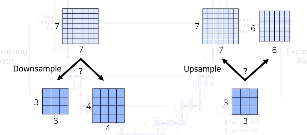
• What is the spacial size of the feature map is an odd number?
  • Downsample 시에는 버림하여 7 -> 3
  • Upsampling 하면 3 -> 6
  • 7에서 6으로 원상복구가 안 됨. 그렇기 때문에 홀수 사이즈의 feature map이 나오지 않게 해야 함.
    

DeepLab

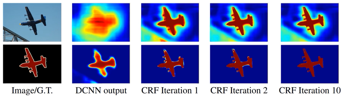
• Conditional Random Fields (CRFs)
  • 후처리의 일종
  • CRF post-processes a segmentation map to be refined to follow image boundaries
  • 1st row : score map (before softmax) / 2nd row : belief map (after softmax)
    
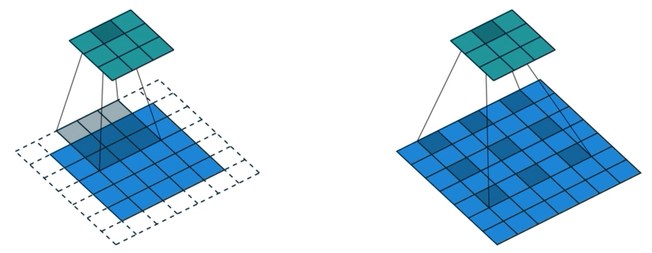
• Dilated Convolution
  • Atrous convolution
  • Inflate the kernel by inserting spaces between the kernel element (Dilation factor)
  • Enable exponential expansion of the receptive field
    
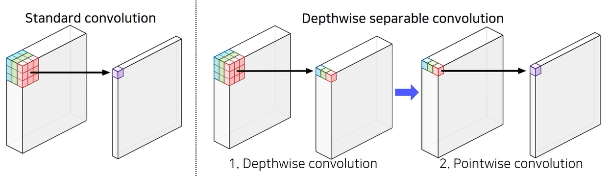
• Depthwise separable convolution
  • Number of parameters
    • Standard Conv : $D_K^2MND_F^2$
    • Depthwise separable conv : $D_K^2MD_F^2 + MND_F^2$
      $D_K/D_F$ : Kernel/Feature map size
      $M/N$ : Input/Output channels
      
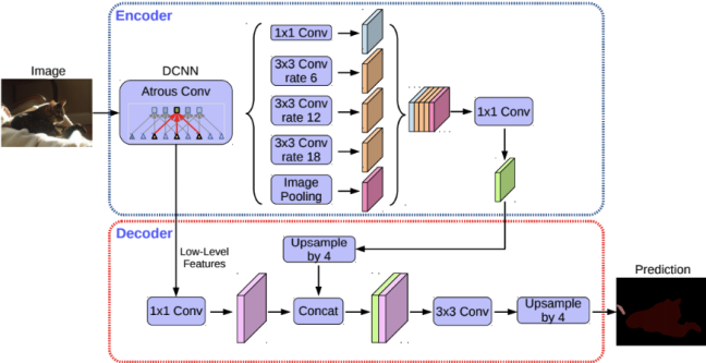
• DeepLap V3+
  • Dilated convolution (=Astrous convolution)
  • Atrous Spatial Separable Pyramid Pooling
    

Object Detection

같은 class라도 다른 object라면 이를 분류해야 한다!

What is object detection

• Classification + Box Localization (Bounding Box) : output = $(p_{class},x_{min},y_{min},x_{max},y_{max})$

Traditional Methods

• Gradient-based detector (e.g., HOG)
  • feature를 사람이 정교하게 엔지니어링하여 디자인하고 머신러닝 알고리즘은 단순한 선형 모델을 사용함.
• Selective Search
  • box propose algorithm
  • Over-segmentation
  • Iteratively merging similar regions
  • Extracting candidate boxes from all remaining segmentations.

Two-stage detector

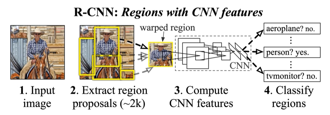
R-CNN

• Directly leverage image classification networks for object detection
  
  • region proposal : Selective Search 등을 이용하여 2000장 정도 region 제안
  • warp : 이미지 사이즈 다시 만들기 (vs resize?)
• Problem : 자르고 CNN에 넣다 보니 2000장에 대해 하기 위해서는 너무 느림. 그리고 selective search가 사람이 design 한 것이다 보니 성능 개선이 어려움.
• Solution : Fast R-CNN

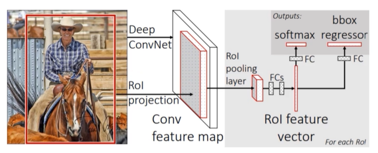
Fast R-CNN

• Recycle a pre-computed feature for multiple object detection
• 1. Conv feagure map from the original image
• 2. RoI(Region of Interest) feature extraction from the feature map through RoI pooling
• 3. Class and box prediction for each RoI
     
• Problem : 여전히 selective search를 통해 RoI를 추출함
• Solution : Faster R-CNN

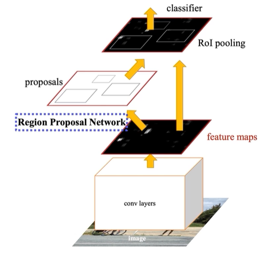
Faster R-CNN

• End-to-end object detection by neural region proposal
• Concept
  • IoU : Intersection over Union. A metric commonly used in object detection.
    $\text{IoU}=\frac{\text{Area of Overlap}}{\text{Area of Union}}$
  • Anchor boxes : A set of pre-defined bounding boxes. 미리 scale 별 ratio 별 다양한 anchor box를 준비해놓고 ground truth와 비교해서 positive, negative sample로 나눈다.
    • IoU with GT > 0.7 -> positive sample
    • IoU with GT < 0.3 -> negative sample
• Time-consuming selective search 대신 Region Proposal Network(RPN) 사용
  
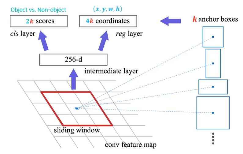
• RPN
  • 이미지가 conv layer를 통과하여 feature map 추출
  • feature map의 각 위치에서 sliding window (논문에서는 3*3 filter 사용)
  • 각 위치에 대해 region proposal을 생성하기 위해 k개의 anchor box를 사용함.
  • cls layer는 k개의 박스에 대해 객체가 있는지 없는지에 대한 2k scores를 출력 (binary)
  • reg layer는 k개의 박스의 좌표 정보인 4k를 출력
  • feature map의 크기가 $W\times H$면 총, $WHK$개의 anchor를 사용함. 각 위치마다 anchor를 이용하여 region proposal을 생성함. 생성된 proposal에는 object score, 4개의 좌표 총 6개의 정보가 있음. 이 proposal이 R-CNN을 거쳐 class 확률을 얻는다.
    
  • Non-Maximum Suppression(NMS)
    • 다양한 anchor box로 학습하기 때문에 한 object에 대해 많은 bounding box가 있을 수 있다. 그 중 잡다한 것은 버려야함.
    • 1. Select the box with the highest objectiveness score
    • 2. Compare IoU of this box with other boxes
    • 3. Remove the bounding boxes with IoU > 50% : 많이 겹칠수록 같은 물체를 검출하고 있다고 판단하기 때문에
    • 4. Move to the next highest objectiveness score
    • 5. Repeat steps 2-4

One-stage detector

No explicit RoI pooling

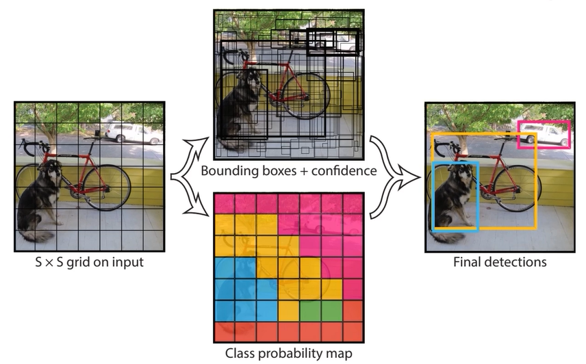
You Only Look Once (YOLO)

• 네트워크외 최종 출력단에서 bounding box와 classification이 동시에 이뤄진다.
  
• Faster R-CNN보다 빠르지만 성능은 조금 떨어짐
• Problem : 맨 마지막에 한번만 prediction을 하기 때문에 localization 정확도가 조금 떨어진다.
• Solution : Single Shot Multibox Detector (SSD)

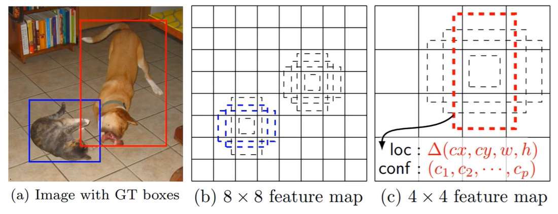
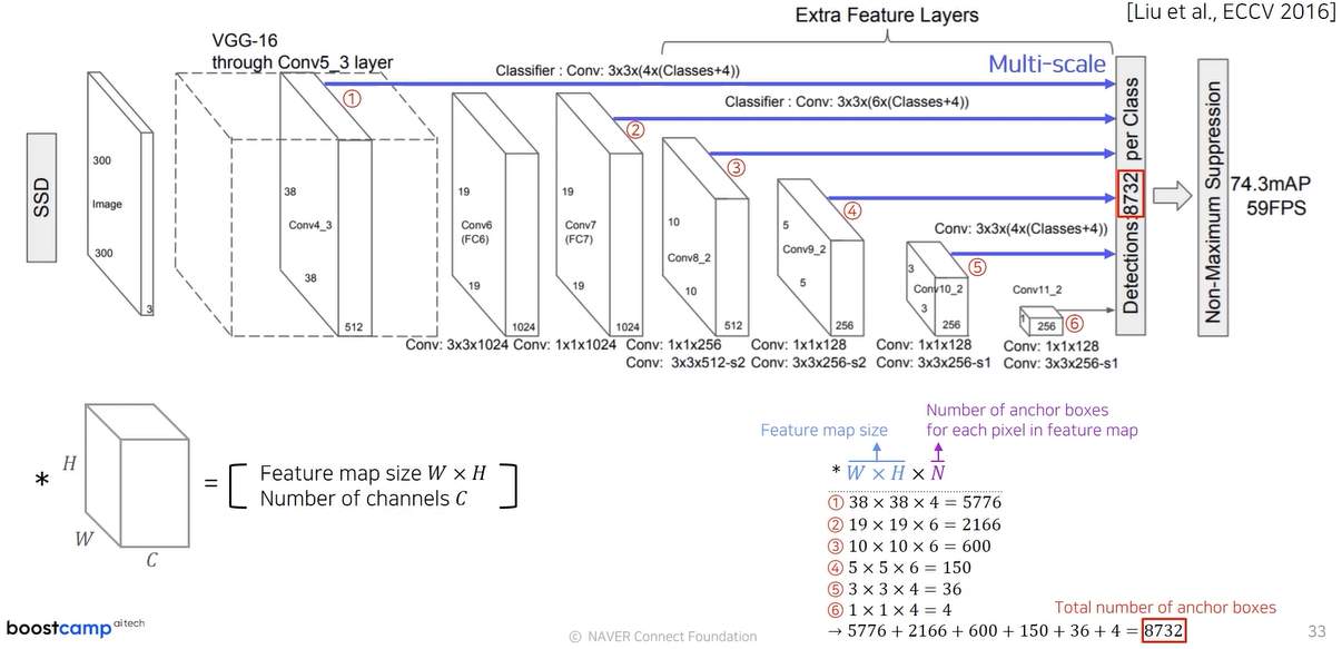
Single Shot Multibox Detector (SSD)

• The use of multi-scale outputs attached to multiple feature maps enable effectively modeling a diverse space of possible box shapes.
• 각 feature map에서 적절한 conv 연산을 통해 우리가 예측하고자 하는 bounding box의 class 점수와 offset을 얻게 됨.
• 
• 
• YOLO보다 빠르고 Faster R-CNN보다 좋은 성능

Two-stage detector vs One-stage detector

• Class imbalance problem
  • 일반적으로 사진에서 배경이 대부분이고 객체는 일부분만을 차지하는 경우가 많음
  • class imbalance : # of neg anchor boxes >> # of pos anchor boxes
  • 이는 one-stage detector에서 문제임
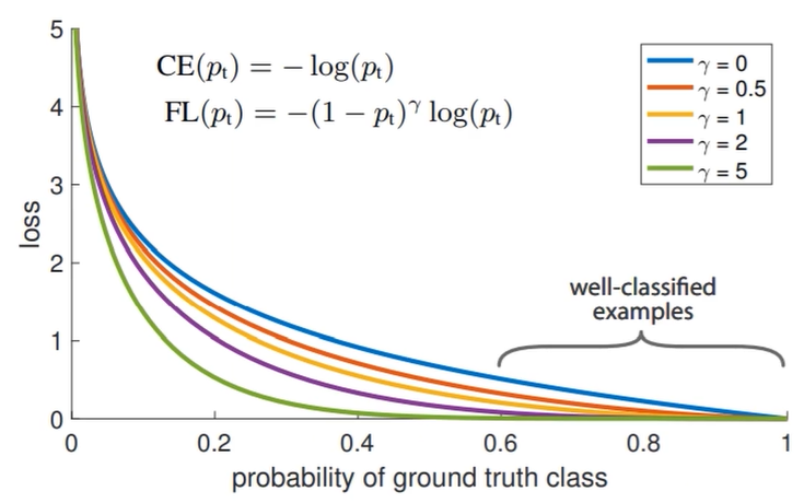
  • Solution : Focal Loss
• Focal Loss : $-(1-p_t)^\gamma \log{p_t}$
  cf) CE Loss : $-\log{p_t}$
  • Improved cross entropy loss
  • Deal with class imbalance
    • Over-weights hard or misclassified examples
    • Down-weights easy examples
      
    • 단순히 loss를 보지 말고 gradient를 보면 $\gamma$가 클수록 sharp한 그래프가 나오게 됨.

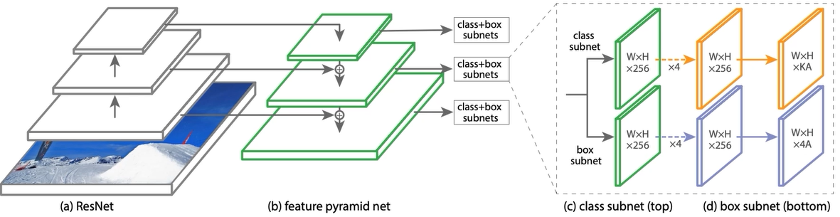
RetinaNet

• One-stage network
• Feature Pyramid Networks(FPN) + class/box prediction branches
  

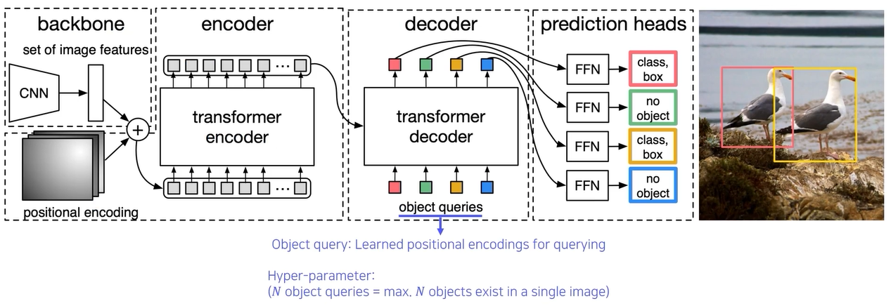
Detection with Transformer

DETR (DEtection TRansformer)

Day 5

강의 듣기 - CNN Visualization

What is CNN Visualization

• CNN is a black box
  • What is inside CNNs (black box)?
  • Why do they perform as well?
  • How would they be improved?

ZFNet

• Deconvolution을 이용해서 CNN의 black box를 보고자 함
• 앞쪽이 feature map에서는 방향성이 있는 feature나 어떤 모양을 가지는 feature를 찾으려 했고,
• 뒤쪽의 feature map일수록 high-level의 의미를 찾으려고 함
• 눈으로 feature map을 보며 tuning 했음.

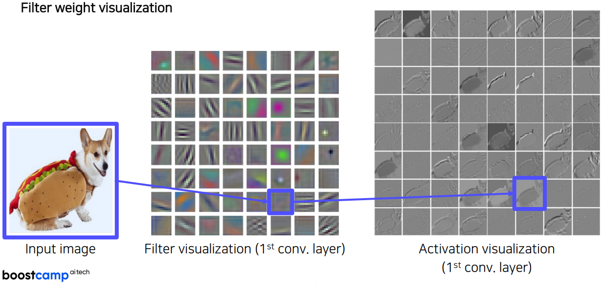
Filter weight visualization

• 어떤 필터냐에 따라 색상을 강조했냐, 고대비를 강조했냐, 색상의 분포를 강조했는지 보는 것
  
• 왜 1st conv layer에 대해서만 확인할까?
  • 뒤쪽 layer는 차원 자체가 높음. visualization 할 수 있는 형태가 아님. 사람이 볼 수 없어 직관적으로 확인할 수가 없음.
  • 앞쪽 layer와 섞여서 더 추상적인 이미지가 나옴.

Analysis of model behaviors

Embedding feature analysis

Nearest neighbors in a feature space

• original image에서 pixel-wise하게 NN을 찾는다면 문제가 있음.
  • 같은 강아지여도 이미지 내의 위치에 따라 다르기도 하고 색깔에 따라 너무 다르기 때문에
• 미리 학습된 Neural Network를 준비함.
• FC layer 이전까지 나온 high-dimensional feature map을 준비함.
• 고차원 feature map에서의 Nearest Neighbor 확인하기

Dimensionality reduction

• 마지막 단의 고차원 feature map은 인간이 직관적으로 확인할 수 없음.
• 3차원 혹은 저차원으로 줄여서 표현하는 방법을 생각해야 함.
• t-SNE 등등...

Activation investigation

Layer Activation

• Behaviors of mit-to-high level hidden units
• Layer의 Activation을 분석함으로써 모델의 특성을 파악
• 어떤 채널은 무엇을 찾는 채널이구나! 를 해석적으로 파악 가능함.

Maximally activating patches

• hidden layer의 한 채널을 가져왔을 때 가장 큰 값을 가지고 있는 부분의 패치를 뜯어 보는 것.
• 어떤 패치가 어떤 특징을 보는지 해석적으로 파악 가능함.
• 1. Pick a channel in a certain layer
• 2. Feed a chunk of images and record each activation value (of the chosen channel)
• 3. Crop image patches around maximum activation values

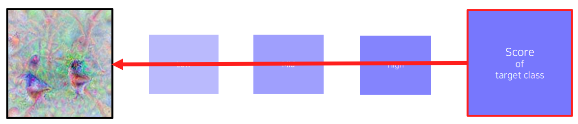
Class Visualization

• Gradient Ascent
• Generate a synthetic image that triggers maximal class activation
  $I^*=\arg\max_{I}f(I)-Reg(I)$
  • $f(I)$ : 어떤 image $I$가 CNN layer $f(.)$를 거쳐 나온 결과값 (score)
  • $I^*$ : 정해진 target으로 만들어진 이미지
  • $Reg(I)$ : Regularization term. $\lambda \|I\|_2^2$
• 1. Get a prediction score (of the target class) of a dummy image (blank or random initial)
• 2. Backpropagate the gradient maximizing the target class score w.r.t the input image
• 3. Update the current image
• 4. redo 1-3
     

Model decision explanation

Saliency test

영상이 주어졌을 때 그 영상이 제대로 판정되기 위한 각 영역의 중요도를 파악하는 것

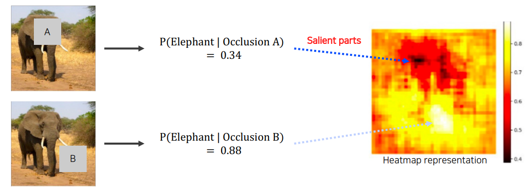
Occlusion map

• 코끼리 이미지가 있다면 그 이미지의 일부를 가리고 neural network에 넣어보고, 코끼리일 확률을 계산해본다.
• 어느 부분을 가리느냐에 따라 확률이 달라질 것이다.
• 그 score를 map으로 나타내어 검은 부분은 코끼리라고 결정하는데 큰 도움이 되는 부분임을 알 수 있음
  

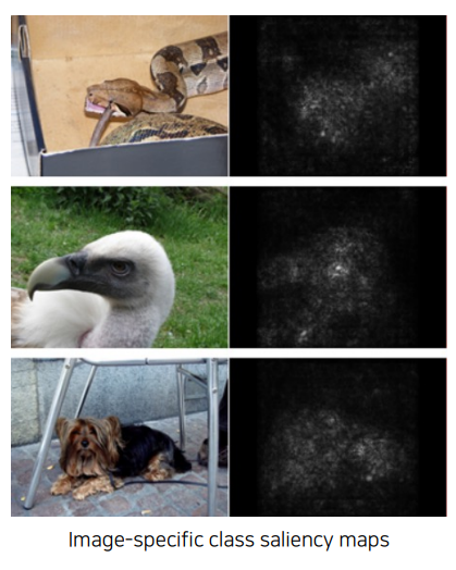
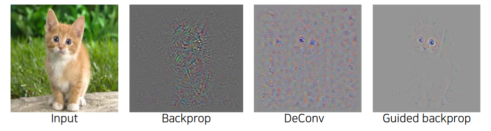
via Backpropagation

• 특정 이미지를 classification 해보고 최종 결론의 class에 결정적인 영향을 미친 부분이 어디인지 heatmap을 그려보는 것.
• 1. Get a class score of the target source image
• 2. Backpropagate the gradient of the class score w.r.t. input domain
• 3. Visualize the obtained gradient magnitude map (optionally, can be accumulated) - gradient의 절대값, 제곱 등을 이용함.
     

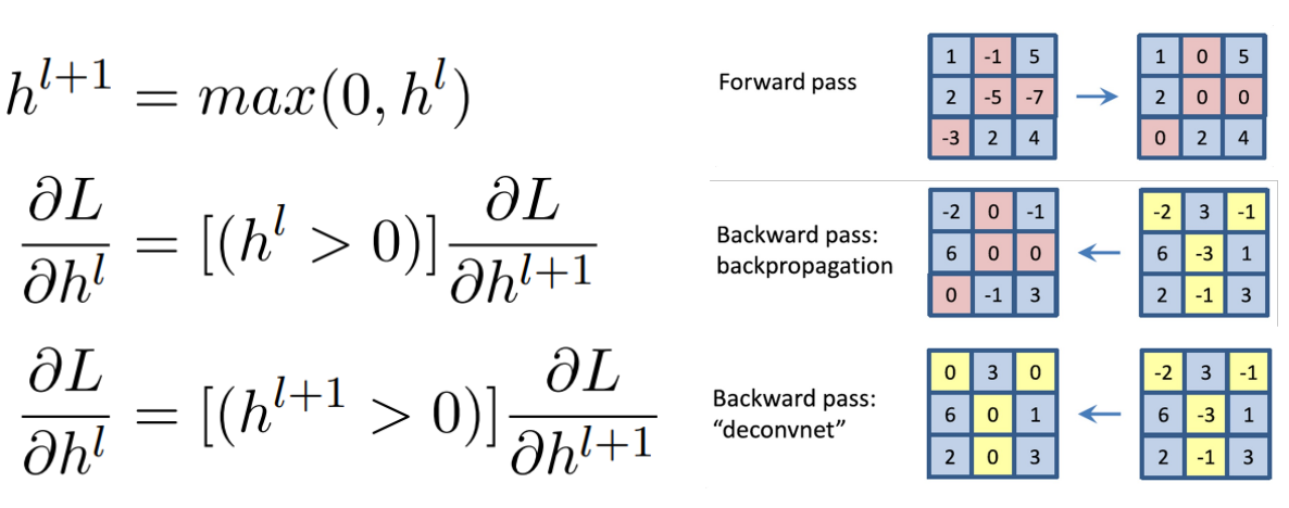
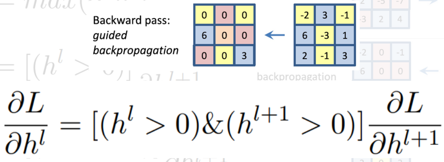
Rectified unit (backward pass)

• Backpropagation based saliency test method
• Deconvolution 시에 ReLU를 적용시켜 gradient가 0이하인 것을 무시하면서 deconvolution을 함.
  
• Guided Backprop이 등장함. forward, backward에서 &(and) gate를 사용하여 backprop
  
• 이는 수학적으로나 의미적으로나 nonsense 하지만 결과론적으로 잘 saliency를 확인할 수 있음.
  

Class Activation Mapping (CAM)

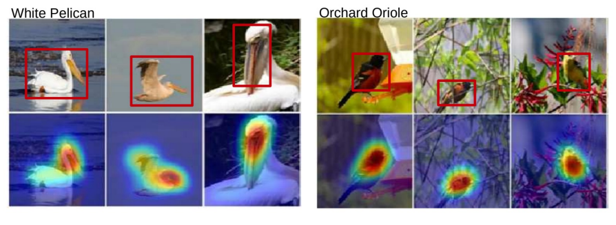
Class Activation Mapping (CAM)

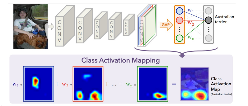
• Visualize which part of image contributes to the final decision
  
• Global Average Pooling (GAP) layer instead of the FC layer
  $S_c = \sum_k w_k^cF_k \xlongequal{GAP}\sum_kw_k^c\sum_{(x,y)}f_k(x,y)$
  위의 연산은 모두 linear하기 때문에 순서를 변경할 수 있다.
  $S_c=\sum_{(x,y)}\sum_k{w_k^cf_k(x,y)}=\sum_{(x,y)}\sum_k\text{CAM}_c(x,y)$
  
• By visualizaing CAM, we can interpret why the network classified the input to that class
• GAP layers enables localizatio without supervision
• 단, 마지막 layer가 GAP + FC layer여야 하고, 그 구조로 학습이 되어야 함. 그나마 ResNet, GoogLeNet은 GAP layer가 있어서 사용하기에 용이함

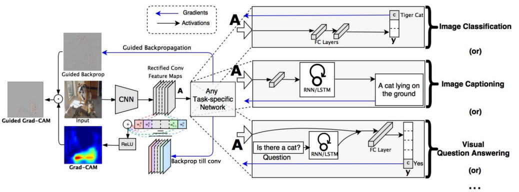
Grad-CAM

• CAM의 단점인, 구조를 변경해야 하며 재학습해야 하는 부분을 보완한 것.
• Backbone이 CNN이기만 하면 어떤 Task든, 어떤 pretrained model이든 상관없이 적용 가능함.
• Get the CAM result without modifying and re-training the original network
• $\text{CAM}_c(x,y) = \sum_k{w_k^cf_k(x,y)}$
  • Key idea : How to obtain the importance weights $w_k^c$?
• Measure magnitudes of gradients as neuron importance weights
• $\alpha_k^c=\frac{1}{Z}\sum_i\sum_j\frac{\partial y^c}{\partial A_{ij}^k}$
  • $\alpha_k^c$ : Importance weight of the k-th feature map w.r.t. the class c
  • $\frac{1}{Z}\sum_i\sum_j$ : Global Average Pooling
  • $\frac{\partial y^c}{\partial A_{ij}^k}$ : Gradients via backprop
• $L_{Grad-CAM}^c=\text{ReLU}(\sum_k\alpha_k^cA^k)$
  
• Guided Backprop과 함께 쓰이기도 함.
• Grad Cam은 smooth, rough하지만 class를 잘 나타낼 수 있고, Guided backprop은 sharp하지만 class 별로 구분하기 힘듦. 그래서 이를 곱해서 사용하면 high-frequency면서 class를 잘 구분할 수 있는 texture map을 구할 수 있다.

SCOUTER

• SCOUTER tells 'why the image is of a certain category?' or 'why the image is not of a certain category.'
• 즉, 이미지가 그 class로 구분된 이유 뿐만 아니라 그 class로 구분되지 않은 이유를 알려줌

Conclusion

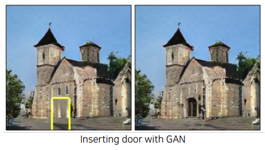
CNN layer에서 왜 그렇게 학습을 했고, 구분을 했는지에 대해 알았던 것을 다른 부분에서도 사용할 수 있음. 그렇게 생각한 것을 토대로 어떤 새로운 것을 만들 수도 있다! -> GAN dissection

• Spontaneously emerging interpretable representation during trianing
• Not only for analysis but also for manipulation applications
  

AutoGrad

Autograd

• Automatic gradient caculating API
• Automatic differentiation is a buioding block of every DL library (forward & backward pass)