Constrained Optimization

Constrained Optimization

General Constrained Optimization

• $f$ : objective function.

• $g_i$ : inequality constraints.

• $h_j$ : equality constraints.

• 제약 조건을 만족하는 $x$의 집합을 feasible set 이라고 한다.

• 점 $x$에 대해 $A(x)=\{i:g_i(x)=0\} \cup \{j:h_j(x)=0\}$을 active set 이라고 한다.

• 주어진 점 $x^*$과 active set $A(x^*)$에 대해, $\{\nabla g_i(x^*), i \in A(x^*)\}$이 linearly independent이면, LICQ (Linearly Independence Constraint Qualification)가 성립한다고 말한다.

LICQ 성립 시, active constraint의 gradient는 0이 될 수 없다.

• The problem can be rewrite as:

• 주어진 문제의 Lagrangian 은 다음과 같이 정의된다.

Karush-Kuhn-Tucker (KKT) Conditions

Motivation for the KKT Conditions

하나의 inequality constraint를 가진 optimization problem을 고려하자.

이는 다음과 같이 표현될 수 있다.

이 때, $f_{\infty-step} = \max\limits_{\lambda \ge 0}$ $L(x,\lambda)$ where $L(x,\lambda)= f(x) + \lambda g(x)$.

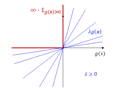
따라서, 해당 optimization problem은 다음과 같이 새롭게 표현될 수 있다:

KKT Conditions

Theorem: First-Order Necessary Conditions (KKT conditions)
Suppose that $x^*$ is a local solution of constrained optimization problem and the LICQ holds at $x^*$.

$\begin{aligned} & \text{minimize} & & f(x) \\ & \text{subject to} & & g_i(x) \le 0, \quad i=1,\dots,l\\ & & & h_j(x) = 0, \quad j=1,\dots,m\\ \end{aligned}$

Then there is a Lagrangian multiplier vector $(\lambda^*, \nu^*)$, such that the following KKT conditions are satisfied at $(x^*, \lambda^*, \nu^*)$:

$\begin{aligned} &\text{(1)} \quad \nabla_x L(x^*,\lambda^*,\nu^*) = \nabla_x f(x^*) + \sum_{i=1}^l\lambda_i^*\nabla_x g_i(x^*) + \sum_{j=1}^m\nu_j^*\nabla_x h_j(x^*) = 0 \\ &\text{(2)} \quad g_i(x^*) \le 0, \forall i \\ &\text{(3)} \quad h_j(x^*) = 0, \forall j \\ &\text{(4)} \quad \lambda_i^* \ge 0, \forall i \\ &\text{(5)} \quad \lambda_i^* g_i(x^*) = 0, \forall i \end{aligned}$

각 조건은 다음과 같이 불린다.

• (1): Stationarity 조건
• (2), (3): Primal feasibility 조건
• (4): Dual feasibility 조건
• (5): Complementary slackness 조건

Lagrangian Duality

Primal and Dual Problem

• Primal problem

or

• Lagrangian Dual problem

Duality Theorem

Weak Duality

Dual problem의 optimal value는 primal problem의 optimal value의 lower bound이다.

Theorem: Weak Duality
Let $x$ and $(\lambda,\nu)$ be a feasible solution to primal and dual problems, respectively.
Then $f(x) \ge D(\lambda,\nu)$.
Moreover, if $f(x^*)=D(\lambda^*,\nu^*)$, then $x^*$ and $(\lambda^*,\nu^*)$ solves the primal and dual problems, respectively.

• Duality gap: $f(x^*)-D(\lambda^*,\nu^*)$

Strong Duality

Convex optimization problem의 경우, dual problem과 primal problem의 optimal value는 같다.

Theorem: Strong Duality
Let $f,g_i$ be convex and $h_j$ be affine for all $i,j$. Then $f(x^*) = D(\lambda^*,\nu^*)$ if the optimal value is finite.

• Affine functions $f(x_1,...,x_n)=A_1x_1+...+A_nx_n+b$ 형태의 function.

Wolfe Duality

Strong Duality를 이용하면 주어진 optimization 문제를 다르게 표현할 수 있다.

Theorem: Wolfe Duality
Let $f,g_i$ be convex, $h_j$ be affine for all $i,j$, and $x^*$ be an optimal solution of the primal.
Then $(x^*,\lambda^*,\nu^*)$ at which LICQ holds solves the Wolfe dual problem of the form

$\begin{aligned} & \text{minimize} & & L(x,\lambda,\nu) \\ & \text{subject to} & & \nabla_xL(x,\lambda,\nu)=0\\ & & & \lambda \ge 0\\ \end{aligned}$

$\nabla_xL(x,\lambda,\nu)=0$는 $L(x,\lambda,\nu)$의 local optima에 대한 조건이다.

Linear and Quadratic Programming

Linear Programming (LP)

• Lagrangian dual $L(x,\lambda,\nu) = c^Tx-\lambda^Tx+\nu^T(b-Ax)$은 convex이다.
• 따라서, $c-\lambda-A^T\nu=0$ and $\lambda\ge 0$ 일 때, minimum을 얻는다.
  * Check that $c-\lambda-A^T\nu=0$ and $\lambda\ge 0$ $\Longleftrightarrow$ $A^T\nu \le c$.
• 그 결과, dual problem은 다음과 같다.

Quadratic Programming (QP)

where $H$ is symmetric and positive semidefinite. (따라서, objective function은 convex이다.)

• Lagrangian dual $L(x,\lambda) = \frac{1}{2}x^THx+d^Tx+\lambda^T(Ax-b)$은 convex이다.
• 따라서, $Hx+A^T\lambda+d=0$ or $x=-H^{-1}(d+A^T\lambda)$ 일 때, minimum을 얻는다.
• 그 결과, dual problem은 다음과 같다.

where $D=-AH^{-1}A$ and $c=-b-AH^{-1}d$.

이 dual problem은 단순히 nonnegative domain에서의 concave quadratic function maximization 문제이기에, 상대적으로 쉽게 풀 수 있다.