Unconstrained Optimization

Theory of Unconstained Optimization

Optimality Conditions

Lemma:
Suppose that $f: \mathbb{R}^n \rightarrow \mathbb{R}$ is differentiable at $\bar{x}$. If there is a vector $d \in \mathbb{R}$ such that $\nabla f(\bar{x})^Td < 0$, then $d$ is a descent direction of $f$ at $\bar{x}$.

• sketch of proof: $f(x+\lambda d) \approxeq f(x) + \lambda \nabla f(x)^Td \le f(x)$ for $\lambda \ge 0$.

추후 나올 Gradient Descent 또는 SGD의 기본 원리이다.

Theorem: First-Order Necessary Optimality Conditions (FONC)
Suppose $f: \mathbb{R}^n \rightarrow \mathbb{R}$ is differentiable at $x^*$.
If $x^*$ is a local minimum, then $\nabla f(x^*) = 0$.

Theorem: Second-Order Optimality Conditions
Suppose $f: \mathbb{R}^n \rightarrow \mathbb{R}$ is twice differentiable at $x^*$.\
[Necessary] If $x^*$ is a local minimum, then $\nabla f(x^*) = 0$ and $\nabla^2 f(x^*)$ is positive semidefinite.\
[Sufficient] If $\nabla f(x^*) = 0$ and $\nabla^2 f(x^*)$ is positive definite, then $x^*$ is a strict local minimum.

Determining Local Optima

1. Find the critical points of $f(x,y)$ by solving the system of simultneous equations: $f_x=0, f_y=0$.

2. Let $D(x,y)=f_{xx}f_{yy} - f_{xy}^2$.

3. Then

   1. $D(a,b)>0$ and $f_{xx}(a,b)<0$ implies that $f(x,y)$ has a local maximum at the point $(a,b)$.

   2. $D(a,b)>0$ and $f_{xx}(a,b)>0$ implies that $f(x,y)$ has a local minimum at the point $(a,b)$.

   3. $D(a,b)<0$ implies that $f(x,y)$ has neither a local maximum nor a local minimum at the point $(a,b)$, it has instead a saddle point.

   4. $D(a,b)=0$ implies that the test is inconclusive, so some other technique must be used to solve the problem.

Line Search Strategy

Line Search

Line search는 numerical analysis에서 (근사) 해를 찾는 기법으로 복잡한 diffrentiable function에 대해 적절하게 사용될 수 있다.

기본적으로 주어진 점 $x_k$에서 search direction $p_k$를 계산하고, 해당 방향으로 positive scalar인 step length $\alpha_k$만큼 이동하여 새로운 점 $x_{k+1}$을 찾는다.

따라서, line search method는 적절한 search direction과 step length를 선택하는 것이 중요하다.

Step length는 일반적인 learning algorithm에서 learning rate와 같다.

$p_k$는 descent direction, i.e. $p_k^T\nabla f_k <0$, 으로 정하는 것이 합리적이며 많은 line search methods에서, $p_k$는 다음과 같은 form을 갖는다.

where $B_k$ is a symmetric and nonsingular matrix.

The Wolfe Conditions

The Wolfe condition은 inexact line search 방법에서 step length를 결정하기 위한 기준을 제공한다.

• [Armijo condition : $f(x_k + \alpha_k d_k) \leq f(x_k) + c_1 \alpha_k \nabla f(x_k)^T d_k$]
  새로운 점에서의 함수 값이 현재 점에서의 값보다 충분히 감소해야 한다.
• [curvature condition : $\nabla f(x_k + \alpha_k d_k)^T d_k \geq c_2 \nabla f(x_k)^T d_k$]
  새로운 점에서의 경사가 원래 경사의 $c_2$배 이상이어야 한다. (너무 멀리 가지 않고, 너무 평평한 구역에 위치하지 않도록 한다.)

Line Search Methods

• Steepest Descent
  • $x_{k+1} = x_k - \alpha_k \nabla f_k$
  • The rate-of-convergence is linear.
  • Global convergence if $\alpha_k$ satisfies the Wolfe conditions.

우리가 흔히 말하는 Gradient Descent 방법이다.

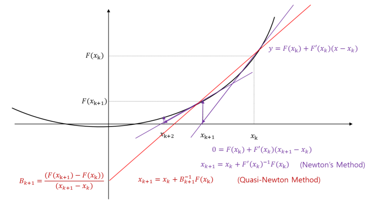
• Quasi-Newton Method

  • $x_{k+1} = x_k - \alpha_k B_k^{-1}\nabla f_k$
  • The rate-of-convergence is superlinear.
  • Global convergence if $\alpha_k$ satisfies the Wolfe conditions.
  • The BFGS method is the most popular.

• Newton's Method

  • $x_{k+1} = x_k - (\nabla^2 f_k)^{-1}\nabla f_k$
  • The rate-of-convergence is quadrtic.
  • Local convergence.