Zhu, Z., Xu, M., Bai, S., Huang, T., & Bai, X. (2019). Asymmetric non-local neural networks for semantic segmentation. In Proceedings of the IEEE/CVF International Conference on Computer Vision (pp. 593-602).
Non-local Series
아래에서 Non-local operation에 대한 내용을 먼저 다루었습니다.
1. Non-local Neural Networks
1. Introduction
@ Long range dependency
현재 많은 연구에서 사용되고 있는 Convolution은 long range dependency를 포착하는 데 제한된 역량을 가지고 있다. 단일 convolution filter는 그 부분에 상관있는 부분을 모두 포착하는 데 receptive field의 크기가 제한적이기 때문이다.
Long range dependency - 한 부분에 대해 상관 관계를 가지는 부분은 꼭 그 부분 근처에 있을 것이란 보장은 없다. 예를 들어 한 사람이 공을 찼을 때 멀리 떨어진 공은 공의 주변의 배경보다는 멀리 떨어진 공을 찬 사람이 더 관련이 있을 것이다. 이렇게 거리적으로 멀리 떨어졌으나 그 두 요소가 가지는 상관관계를 long range dependency라 부른다.
이전의 연구들은 long range dependency를 충분히 활용하는 경우 성능이 개선될 수 있다고 말하고 있다.
@ Non-local
Non-local Neural Networks에서 non-local means라는 컴퓨터 비전에서 image denoising을 위한 filter 테크닉을 신경망과 결합해 이미지 내의 한 위치와 다른 모든 위치들 간의 상관관계를 계산했다.

하지만 이 Non-local operation을 거치는 과정에서 많은 컴퓨팅 비용과 GPU 메모리 점유가 필요했다. 본 논문의 저자들은 Key branch와 Value branch에서의 출력 크기가 동일하다면 non-local block의 출력 크기가 변하지 않을 것이라고 생각했다.
이에 따라 Key branch와 Value branch에서 몇 가지 대표적인 지점()만 샘플링할 수 있으면 컴퓨팅 비용을 크게 줄일 수 있다고 제안한다.
2. Related Work
Semantic segmentation과 scene parsing에서 context information 및 long range dependency를 확보하기 위한 최근 관련 연구를 리뷰한다.
@ Encoder-Decoder
- Long et al., Noh et al.
- FCN의 형태로 Encoder에서 bottleneck feature를 만듬.
- 이를 deconvolution과 같은 방법으로 Decoding하여 sementic segmentation을 수행
- Ronneberger et al.
- U-Net.
- Zhang et al.
- Context Encoding Module을 도입하여 semantic 클래스 중요도를 예측.
- 이를 기반으로 선택적으로 클래스 별 feature map을 강화하거나 약화시킴.
@ CRF
머신러닝에서 주로 context information을 포착하기 위해 frequently-used operation, Conditional Random Field (CRF)를 딥러닝에 결합하는 연구들이 있었다.
- Zheng et al.
- CRF-CNN
- Chandra et al., Vemulapalli et al.
- integrating Gaussian Conditional Random Fields into CNN
@ Different Convolutions
- Chen et al.
- DeepLab, dilated convolutions 적용
- Peng et al.
- large kernel convolutions 적용
@ Spatial Pyramid Pooling
object detection에서 활용되던 spatial pyramid pooling에 영감을 얻어 이를 semantic segmentation에 적용하고자 하는 연구들이 있었다.
- Chen et al.
- DeepLab, multiple scales를 포착하기 위한 Atrous Spatial Pyramid Pooling (ASPP) layer 도입.
- Zhao et al.
- PSPNet
- 서로 다른 scale의 embed context features를 반영하기 위한 Specific layer를 도입.
- Spatial Pyramid Pooling 뒷 부분에 Specific layer 추가
@ Non-local
- Wang et al.
- Non-local means라는 컴퓨터 비전에서 image denoising을 위한 filter 테크닉을 신경망과 결합
- 이미지 내의 한 위치와 다른 모든 위치들 간의 상관관계를 계산
3. Asymmetric Non-local Neural Network
3.1. Revisiting Non-local Block
여기에선 기존의 Non-local Neural Networks의 non-local operation의 설계를 다시 짚어보고 있다.

1.
입력 가 주어졌을 때, convolution 를 통해 를 서로 다른 임베딩으로 변환한다.
는 변환된 임베딩의 채널 수
2.
다음으로 행렬 와 를 의 사이즈로 flatten을 거치고 곱해 행렬 를 생성한다.
즉,
3.
를 Non-local Neural Networks에서 언급한 방법처럼 normalization( function)을 거친다. 여기에서는 softmax, rescaling, none등의 선택지가 있는데 본 논문에서는 softmax(embedded gaussian)를 선택했다.
4.
를 곱한다.
5.
최종 Output은 convolution 를 곱하여 에서 원래 채널 수 로 채널 수를 복원하고 Residual 구조처럼 입력 값 를 더한 값으로 한다.
혹은 입력 와 최종 결과를 concatenate한다.
3.2. Asymmetric Pyramid Non-local Block
위에서 서술한 Non-local network은 long range dependency를 포착하는 데에는 효과적이지만 시간적으로, 메모리적으로 매우 부담되는 연산이다.
@ Motivation and Analysis.
Semantic segmentation에선 세밀한 features를 뽑아내기 위해 큰 해상도의 output을 갖는 경우가 많다. 이 경우 의 시간 복잡도는 굉장한 부담으로 작용한다.
본 논문의 연구진은 단순하게 의 숫자를 더 작은 숫자 로 의 일부를 샘플링하여 줄이는 것으로 해결하고자 했다 .
@ Solution.
위에서의 분석을 토대로 에서 일부 를 sampling하는 모듈인 를 각각에 대해 정의한다.
이후 절차는 기존 non-local block에서와 동일하다.
위와 같은 asymmetric matrix multiplication은 계산 복잡도 면에서 로 기존 non-local block 보다 으로 눈에 띄게 낮은 모습을 볼 수 있다.
@ Asymmetric Pyramid Non-local Block.
그렇다면 전체 에서 일부 를 샘플링하는 방법은 어떻게 되는가?
논문의 저자들은 Global and multi-scale representations를 잡아내는 것에 효과적인 Spatial Pyramid Pooling을 Non-local block에도 적용할 수 있을 것이라는 생각을 했다.
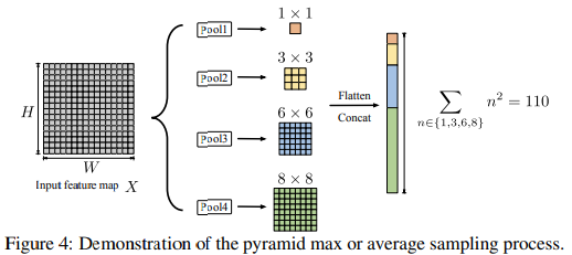
논문에서는 와 에서 각각 네 개의 pooling 결과를 flatten하여 ()로 하였다.
3.3. Asymmetric Fusion Non-local Block
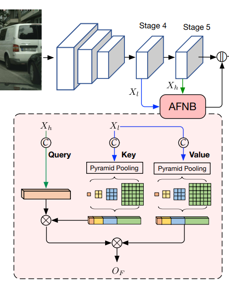
addition이나 concatenate와 같은 방식으로 다른 수준(level)의 두 요소를 fusion하는 것은 semantic segmentation에 좋은 영향을 줄 수 있다.
1.
기존 Non-local block이 하나의 feature map을 입력으로 하는 반면에 Fusion Non-local Block은 두 가지의 입력이 있다.
- low-level feature map:
- : low-level feature map의 크기
- high-level feature map:
- : high-level feature map의 크기
먼저 이 두 가지 입력을 각각의 convolution 임베딩()을 거쳐 임베딩으로 만들어준다.
2.
이 두 행렬을 곱해 유사도 행렬 를 만들고, 동일하게 normalization 과정을 거친다.
3.
다음으로 low-level feature map과 곱해준다.
4.
마지막으로 Residual 과정을 거치고 high-level feature map의 채널 수 로 만들기 위해 convolution을 거친다.
PNB에서 적용했던 것처럼 Fusion Non-local Block에도 spatial pyramid pooling을 적용해 계산량 부담을 완화하였다. 이로인해 각각 Asymmetric PNB(APNB), Asymmetric FNB(AFNB)로 명명했다.
3.4. Network Architecture
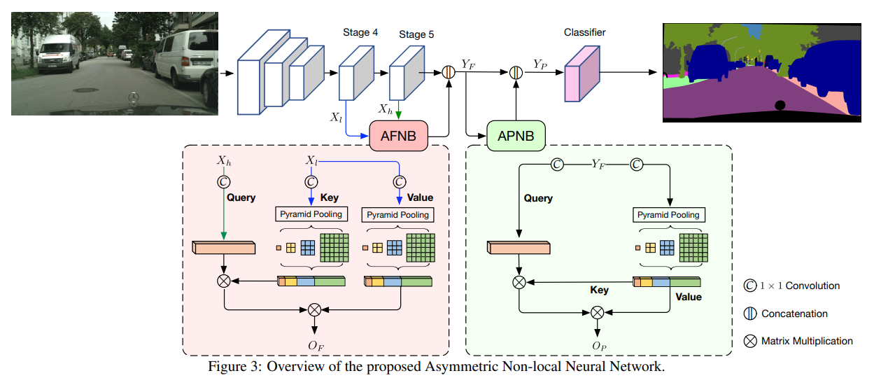
논문에서 ResNet101을 backbone network로 사용했으며 마지막 두 down-sampling 구간을 dilation convolution으로 대체했다. 이는 마지막 두 down-sampling 구간에서의 결과 feature map 크기를 동일하게 유지하기 위함이다. 결과적으로 그림 3에서 볼 수 있듯이 Stage 4, Stage 5, Classifier는 모두 같은 크기를 유지하고 있음을 알 수 있다.
4. Experiments
4.1. Datasets and Evaluations Metrics
@ Datasets
- Cityscapes
- ADE20K
- PASCAL Context
@ Evaluation Metric
- Mean IoU: Mean of class-wise intersection over union
4.2. Implementation Details
@ Training objectives
본 실험에서 사용한 손실함수는 아래와 같이 두 cross entropy loss로 이루어져 있다.
이와 같이 손실함수를 구성한 배경에 대해선 논문에서 서술하고 있지 않지만 기존의 ResNet101의 일부 segmentation 성능을 가져가고 싶은 것 같다.
@ etc.
ResNet101backbone pretrained onImageNetStochastic Gradient Descentoptimizer- learning rate
- initial learning rate
- Cityscapes: 0.01
- PASCAL Context, ADE20K: 0.02
- learning rate decay: ,
- initial learning rate
- Data
- input size, batch size, epochs
- Cityscapes:
- PASCAL Context:
- ADE20K:
- augmentation
- random scaling in the range of
- random horizontal filp
- random brightness
- input size, batch size, epochs
4.4. Ablation Study
@ Efficacy of the APNB and AFNB
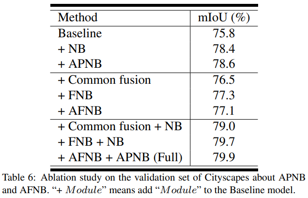
- Baseline:
FCN-like ResNet-101 - + NB:
Classifier이전에 Non-local block 추가 - + Common Fusion: Baseline에서
Stage4->Stage5과정을
Stage5ReLU(BatchNorm(Conv(Stage4)))로 변경
@ Selection of Sampling Methods
APNB 모듈에서 샘플링 방법의 선택은 그 성능에 많은 영향을 미친다.
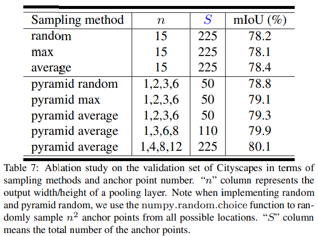
@ Influence of the Anchor Points Numbers
APNB 모듈에서 pyramid pooling layer의 크기 역시 그 성능에 큰 영향을 미친다. Table 7에서처럼 의 크기가 늘어날수록 성능이 향상되는 것 을 볼 수 있으며 논문에서 저자들은 efficacy와 efficiency의 적절한 지점인 을 default setting으로 설정했다.
