이번에 따라할 글은 EDA To Prediction(DieTanic)이다. EDA 부터 prediction까지의 과정을 설명한 글인데 처음 튜토리얼에서 EDA를 자세히 뜯어보았기 때문에 추가로 고려할만한 사항을 간단히 짚고 EDA 후 과정을 중점적으로 다루기로 했다.
Missing Value Handling
train data와 test data에 missing value(결측값)이 있는데 그중 상당수가 나이(age)이다. 이전 글에서는 median으로 통일하여 메꾸긴 했지만 사람의 연령대를 추정할 수 있는 정보가 있다면 최대한 활용하는 것이 좋다. 가령 'name' feature 값에 있는 Miss, Mrs, Mr 같은 단어가 힌트가 된다.
train_data['Initial'] = 0
for i in train_data:
	train_data['Initial'] = train_data.Name.str.extract('([A-Za-z]+\.')
string 값에서 Miss, Mrs, Mr 같은 단어만 추출하기 위해 regex를 쓴다. 보통 Miss, Mrs를 쓸 때 Miss. Sarah, Mrs. Smith처럼 뒤에 '.'을 붙이는데 이를 규칙으로 사용한다. extract의 parameter로 들어가는 '([A-Za-z]+.'가 여기에 해당한다.
Initial이라는 이름을 가진 새로운 feature를 확인해보면 놀랍게도 age값이 null인 record 모두 initial이 잘 뽑힌다. 그리고 종류가 20개보다 적다. (심지어 몇개는 오타로 추정된다.)
EDA to Prediction 글에서 replace한 대로 initial feature를 더 간단하게 만들어보자.
train_data['Initial'].replace(['Mlle','Mme','Ms','Dr','Major','Lady','Countess','Jonkheer','Col','Rev','Capt','Sir','Don', 'Dona'],['Miss','Miss','Miss','Mr','Mr','Mrs','Mrs','Other','Other','Other','Mr','Mr','Mr', 'Mrs'],inplace=True)
train_data.groupby('Initial')['Age'].mean()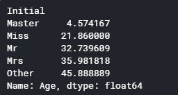
Initial 별로 뽑은 평균으로 null 값을 대체하면 더 잘 보정할 수 있을 것 같다. (Master 호칭이 평균이 4살인데 내가 아는 마스터랑 다른건가)
train_data.loc[(train_data.Age.isnull())&(train_data.Initial=='Mr'),'Age']=33
train_data.loc[(train_data.Age.isnull())&(train_data.Initial=='Mrs'),'Age']=36
train_data.loc[(train_data.Age.isnull())&(train_data.Initial=='Master'),'Age']=5
train_data.loc[(train_data.Age.isnull())&(train_data.Initial=='Miss'),'Age']=22
train_data.loc[(train_data.Age.isnull())&(train_data.Initial=='Other'),'Age']=46
결측값을 채우기 위해 initial이라는 새로운 feature를 만든 김에 이 feature가 생존 확률과 연관이 있을지 겸사겸사 체크해보자.
f, ax = plt.subplots(1, 2, figsize=(20, 10))
train_data[['Initial', 'Survived']].groupby(['Initial']).mean().plot.bar(ax=ax[0])
ax[0].set_title('Survived vs Initial')
sns.countplot('Initial', hue='Survived', data=train_data, ax=ax[1])
ax[1].set_title('Initial: Survived vs Dead')
plt.show()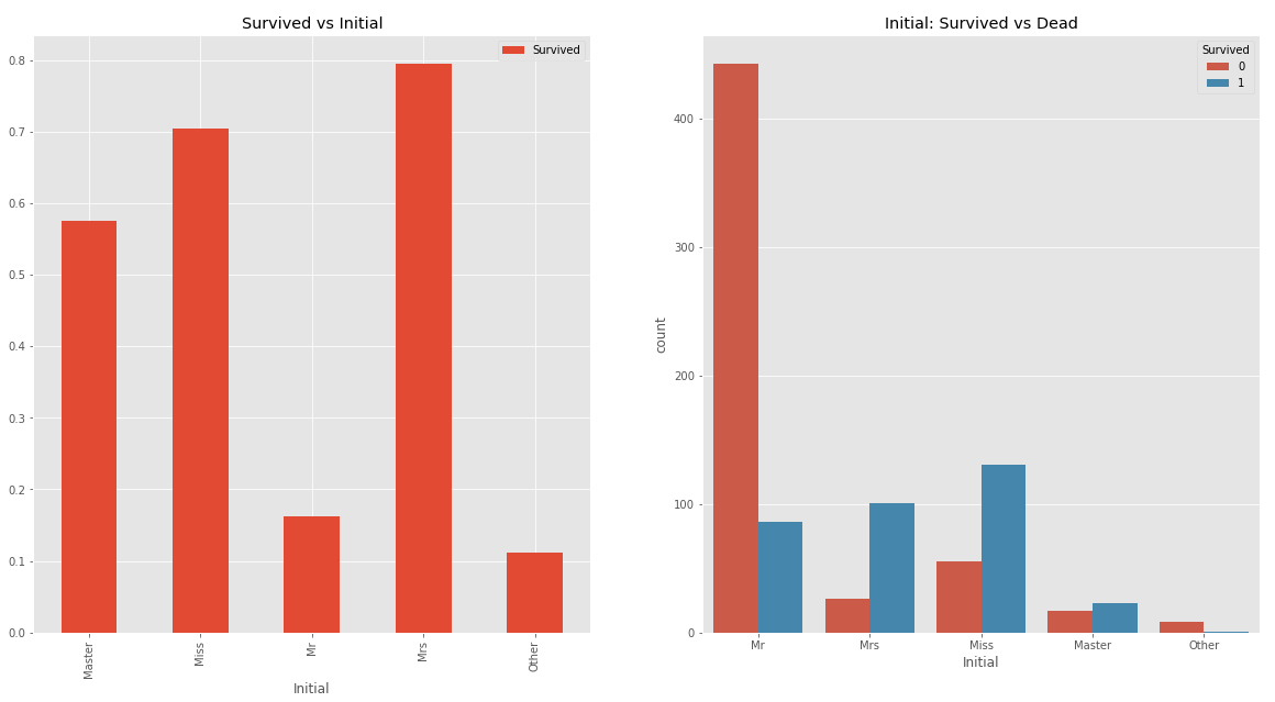
여자를 뜻하는 Miss, Mrs와 평균나이가 어린 Master의 생존 확률이 높다. 이전 글에서 여성과 아이의 생존 확률이 높다는 것을 이미 확인했기 때문에 Initial feature를 분석에 사용해도 괜찮을 것 같다.
Sex, Embarked처럼 feature value가 string이기 때문에 numeric value로 치환한다.
train_data['Initial'] = train_data['Initial'].map({'Mr': 0, 'Mrs': 1, 'Miss': 2, 'Master': 3, 'Other': 4})이 글에서는 embarked, initial feature에 대해 one-hot encoding을 하지 않아서 이번 실습에서도 하지 않았다.
Predictive Modeling
이 글에서는 classification algorithm 여러개를 사용했다.
1. Logistic Regression
2. Support Vector Machine(Linear and radial)
3. Random Forest
4. K-Nearest Neighbours
5. Naive Bayes
6. Decision Tree
앞 글에서 했듯이 train set, valid set으로 나누어서 algorithm마다 accuracy 체크를 해본다.
# radial svm
model = svm.SVC(kernel='rbf', C=1, gamma=0.1)
model.fit(X_tr, y_tr)
prediction1 = model.predict(X_vld)
print ('Accuracy for rbf SVM is ', metrics.accuracy_score(prediction1, y_vld))

# linear svm
model = svm.SVC(kernel='linear', C=1, gamma=0.1)
model.fit(X_tr, y_tr)
prediction2 = model.predict(X_vld)
print ('Accuracy for linear SVM is ', metrics.accuracy_score(prediction2, y_vld))

# logistic regression
model = LogisticRegression()
model.fit(X_tr, y_tr)
prediction3 = model.predict(X_vld)
print ('Accuracy for Logistic Regression is ', metrics.accuracy_score(prediction3, y_vld))

# Decision Tree
model = DecisionTreeClassifier()
model.fit(X_tr, y_tr)
prediction4 = model.predict(X_vld)
print ('Accuracy for Logistic Regression is ', metrics.accuracy_score(prediction4, y_vld))

# K-Nearest Neighbours(KNN)
model = KNeighborsClassifier()
model.fit(X_tr, y_tr)
prediction5 = model.predict(X_vld)
print ('Accuracy for Logistic Regression is ', metrics.accuracy_score(prediction5, y_vld))

# Naive Bayes
model = GaussianNB()
model.fit(X_tr, y_tr)
prediction6 = model.predict(X_vld)
print ('Accuracy for NaiveBayes is ', metrics.accuracy_score(prediction6, y_vld))

# Random Forest
model = RandomForestClassifier(n_estimators=100)
model.fit(X_tr, y_tr)
prediction7 = model.predict(X_vld)
print ('Accuracy for Random Forests is ', metrics.accuracy_score(prediction7, y_vld))| Algorithm | Accuracy |
|---|---|
| Random Forests | 0.8208955223880597 |
| Radial SVM | 0.8171641791044776 |
| K-Nearest Neighbours | 0.8059701492537313 |
| Logistic Regression | 0.7985074626865671 |
| Linear SVM | 0.7947761194029851 |
| Decision Tree | 0.7910447761194029 |
| Naive Bayes | 0.7835820895522388 |
Accuracy는 78~82 정도로 나왔다. Random Forests algorithm의 accuracy가 가장 높으니 random forest를 쓰자!라고 바로 결론을 내릴 수는 없다. 여기서 측정한 accuracy는 train/valid data를 사용한 값이다. 예측 모델이란 게 결국 train하지 않은 새 데이터를 보고 예측하는 것이기 때문에 무작정 높은 accuracy를 갖는 모델을 선정했다간 overfitting이 발생할 수 있다.
Overfitting을 피할 수 있는 방법으로 cross validation이 있다.
Cross Validation
Cross validation은 valid set을 바꿔가며 accuracy를 체크하는 방법이라고 생각하면 된다. train_data에서 train set과 valid set으로 나누는 코드를 다시 살펴보자.
X_tr, X_vld, y_tr, y_vld = train_test_split(X_train, target_label, test_size=0.3, random_state=0)이 코드에서 test_size=0.3의 의미는 train data 중에서 0.3만큼의 subset을 valid set으로 뺀다는 뜻이다. test_size가 0.2이면 5개의 subset이 만들어진다.
여기서 cross validation을 사용하면, 각각의 subset이 돌아가면서 한 번씩 valid set 역할을 담당하게 된다.
Group 1, Group 2, Group 3, Group 4, Group 5, 총 5개의 subset이 있다고 가정하면,
Trial 1: valid set(Group 1), train set(Group 2, 3, 4, 5)
Trial 2: valid set(Group 2), train set(Group 1, 3, 4, 5)
....
Trial 5: valid set(Group 5), trani set(Group 1, 2, 3, 4)
각 trial마다 accuracy를 계산하고 평균을 내던가 해서 좀더 generalised model을 만들 수 있다.
K-fold cross validation이라고 부르는데 여기서 K=subset의 개수로 보면 된다. 위의 예시에서 K=5이다.
K-fold cross validation은 sklearn에서 KFold로 기능을 제공한다.
from sklearn.model_selection import KFold
from sklearn.model_selection import cross_val_score
from sklearn.model_selection import cross_val_predict
kfold = KFold(n_splits=10)
xyz=[]
accuracy=[]
std=[]
classifiers = ['Linear SVM', 'Radial SVM', 'Logistic Regression', 'KNN', 'Decision Tree', 'Naive Bayes', 'Random Forest']
models = [svm.SVC(kernel='linear'), svm.SVC(kernel='rbf'), LogisticRegression(), KNeighborsClassifier(n_neighbors=8), DecisionTreeClassifier(), GaussianNB(), RandomForestClassifier(n_estimators=100)]
for i in models:
    model = i
    cv_result = cross_val_score(model, X_train, target_label, cv = kfold, scoring = 'accuracy')
    cv_result = cv_result
    xyz.append(cv_result.mean())
    std.append(cv_result.std())
    accuracy.append(cv_result)
new_models_dataframe2 = pd.DataFrame({'CV Mean': xyz, 'Std': std}, index=classifiers)
new_models_dataframe2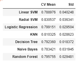
plt.subplots(figsize=(20, 10))
box = pd.DataFrame(accuracy, index=[classifiers])
box.T.boxplot()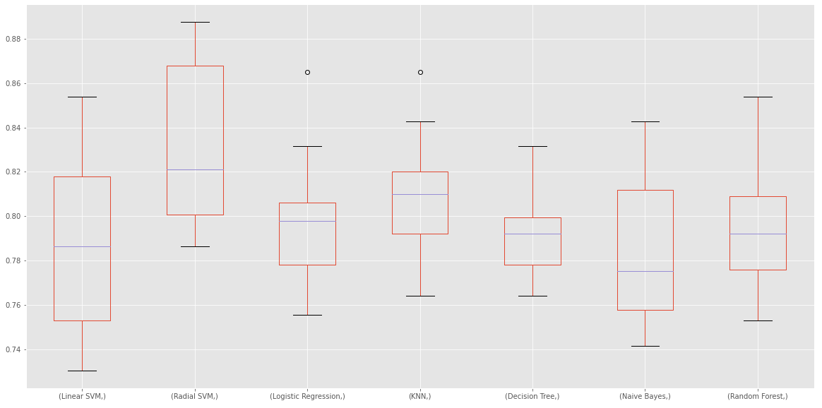
new_models_dataframe2['CV Mean'].plot.barh(width=0.8)
plt.title('Average CV Mean Accuracy')
fig=plt.gcf()
fig.set_size_inches(8,5)
plt.show()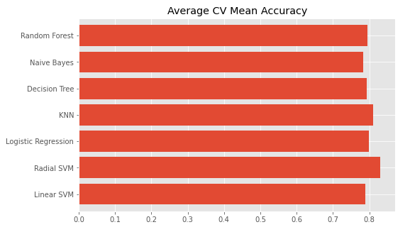
Hyper-Parameter Tuning
Algorithm과 함께 모델의 성능을 좌지우지 하는 것이 hyperparameter이다. K-Fold CV를 할 때 사용한 모델의 hyperparameter를 default 값으로 설정했지만 hyperparameter를 변경하면 accuracy 값도 바뀐다.
EDA to Prediction 글에서는 SVM과 RandomForests가 accuracy가 높아서 이 둘을 hyperparameter tuning했는데 내 경우에는 SVM과 KNN이 가장 높아서 SVM, KNN, RandomForests 세 가지에서 hyperparameter tuning을 해보려 한다.
from sklearn.model_selection import GridSearchCV
# SVM
C = [0.05, 0.1, 0.2, 0.3, 0.25, 0.4, 0.5, 0.6, 0.7, 0.8, 0.9, 1]
gamma = [0.1, 0.2, 0.3, 0.4, 0.5, 0.6, 0.7, 0.8, 0.9, 1.0]
kernel = ['rbf', 'linear']
hyper = {'kernel':kernel, 'C':C, 'gamma':gamma}
gd = GridSearchCV(estimator=svm.SVC(), param_grid=hyper, verbose=True)
gd.fit(X_train, target_label)
print (gd.best_score_)
print (gd.best_estimator_)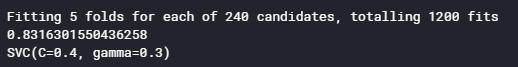
# RandomForest
n_estimators = range(100, 1000, 100)
max_depths = range(3, 8, 1)
hyper = {'n_estimators': n_estimators, 'max_depth': max_depths}
gd = GridSearchCV(estimator=RandomForestClassifier(random_state=0), param_grid=hyper, verbose=True)
gd.fit(X_train, target_label)
print (gd.best_score_)
print (gd.best_estimator_)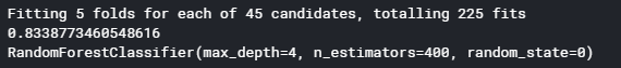
# KNN
n_neighbors = range(1, 20, 1)
hyper = {'n_neighbors': n_neighbors}
gd = GridSearchCV(estimator=KNeighborsClassifier(), param_grid=hyper, verbose=True)
gd.fit(X_train, target_label)
print (gd.best_score_)
print (gd.best_estimator_)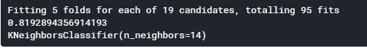
Parameter tuning 결과, RandomForest의 최고치는 max_depth=4, n_estimators=400, random_state=0일 때 accuracy=0.834이다. SVM은 kernel=radial, C=0.4, gamma=0.3일 때 accuracy=0.832이다. KNN은 n_neighbors=14일 때 accuracy=0.819이다.
Ensembling
Algorithm 하나로만 modeling해도 accuracy가 높게 나왔는데 만약 이들을 잘 조합하면 accuracy가 더 높게 나올까? 이와 관련한 개념이 ensembling이다. Ensembling하는 방법에는 voting classifier, bagging, boosting이 있다.
Voting Classifier
여러 machine learning model을 조합하는데 가장 간단한 방법이다. Voting Classifier는 평균 예측 결과를 준다.
from sklearn.ensemble import VotingClassifier

ensemble_lin_rbf=VotingClassifier(estimators=[('KNN',KNeighborsClassifier(n_neighbors=14)),
                                              ('RBF',svm.SVC(probability=True,kernel='rbf',C=0.4,gamma=0.3)),
                                              ('RFor',RandomForestClassifier(n_estimators=400,max_depth=4,random_state=0)),
                                              ('LR',LogisticRegression(C=0.05)),
                                              ('DT',DecisionTreeClassifier(random_state=0)),
                                              ('NB',GaussianNB()),
                                              ('svm',svm.SVC(kernel='linear',probability=True))
                                             ],
                       voting='soft').fit(X_tr,y_tr)
print('The accuracy for ensembled model is:',ensemble_lin_rbf.score(X_vld,y_vld))
cross=cross_val_score(ensemble_lin_rbf,X_train,target_label, cv = 10,scoring = "accuracy")
print('The cross validated score is',cross.mean())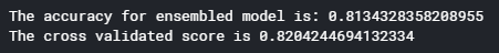
ensembled model accuracy=0.813이고, CV accuracy=0.820이다.
Bagging
Bagging은 보편적으로 쓰이는 방법이다. Sample을 여러번 뽑아 각 모델을 학습시켜 결과를 낸다를 낸다. Variance를 감소하는 방법이라고 생각하면 된다. 그래서 high variance인 model에서 효과가 좋다. 일반적으로 Random Forests나 n_neighbors가 작은 KNN일 때 사용한다고 한다.
from sklearn.ensemble import BaggingClassifier

bagging_model = BaggingClassifier(base_estimator=RandomForestClassifier(max_depth=4), n_estimators=400, random_state=0)
bagging_model.fit(X_tr, y_tr)
prediction_bagging = bagging_model.predict(X_vld)
print ('The accuracy for bagged Random Forests is:', metrics.accuracy_score(prediction_bagging, y_vld))
result = cross_val_score(bagging_model, X_train, target_label, cv=10, scoring='accuracy')
print ('The cross validated score for bagged Random Forests is:', result.mean())
Bagged Random Forests accuracy=0.825가 나왔다. (CV 결과는 running time 너무 길어서 캔슬함)
Boosting
Boosting은 예측하지 어려운 것을 맞추는데 특화된 방법이다. 예측을 반복하면서 이전 회차에 잘못 예측된 결과에 가중치를 두어 예측 결과를 고치려고 한다.
# AdaBoost(Adaptive Boosting)
from sklearn.ensemble import AdaBoostClassifier
ada = AdaBoostClassifier(n_estimators=200, random_state=0, learning_rate=0.1)
result = cross_val_score(ada, X_train, target_label, cv=10, scoring='accuracy')
print ('The cross validated score for AdaBoost is:', result.mean())
AdaBoost accuracy=0.820이다.
Stochastic Gradient Boosting
from sklearn.ensemble import GradientBoostingClassifier
grad = GradientBoostingClassifier(n_estimators=500, random_state=0, learning_rate=0.1)
result = cross_val_score(grad, X_train, target_label, cv=10, scoring='accuracy')
print ('The cross validated score for Gradient Boosting is:', result.mean())

Gradient Boosting accuracy=0.832이다.
# XGBoost
import xgboost as xg
xgboost = XGBClassifier(n_estimators=900, learning_rate=0.1)
result = cross_val_score(xgboost, X_train, target_label, cv=10, scoring='accuracy')
print ('The cross validated score for XGBoost is:', result.mean())
XGBoost accuracy=0.806이다.
Hyper-parameter tuning for Gradient Boosting
Gradient Boosting이 accuracy가 가장 높으므로 이 모델에 대해 hyperparameter tuning을 해보겠다.
n_estimators=list(range(100,1100,100))
learn_rate=[0.05,0.1,0.2,0.3,0.25,0.4,0.5,0.6,0.7,0.8,0.9,1]
hyper={'n_estimators':n_estimators,'learning_rate':learn_rate}
gd=GridSearchCV(estimator=GradientBoostingClassifier(),param_grid=hyper,verbose=True)
gd.fit(X_train,target_label)
print(gd.best_score_)
print(gd.best_estimator_)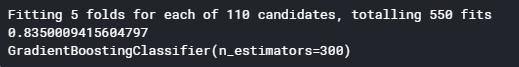
Hyperparameter tuning 결과 n_estimator=300가 나왔다. 이 때 score는 0.835이다.