
6.1 파이프라인을 사용한 효율적인 워크플로
6.1.1 위스콘신 유방암 데이터셋
위스콘신 유방암 데이터셋 - 악성과 양성인 종양 세포 샘플 569개
- 첫 2열 : 샘플의 고유 ID 번호와 진단 결과(M=악성,B=양성)
- 3~32번째 열 : 세포 핵의 디지털 이미지에서 계산된 30개의 실수 값 특성 => 종양이 악성인지 양성인지 예측하는 모델 만들기
☑️pandas를 사용하여 UCI 서버에서 직접 데이터셋을 읽어들임☑️
import pandas as pd

df = pd.read_csv('https://archive.ics.uci.edu/ml/'
                 'machine-learning-databases'
                 '/breast-cancer-wisconsin/wdbc.data', header=None)
☑️30개의 특성을 넘파이 배열 X에 할당☑️
LabelEncoder 객체 : 클래스 레이블을 원본 문자열 표현에서 정수로 변환
from sklearn.preprocessing import LabelEncoder

X = df.loc[:, 2:].values
y = df.loc[:, 1].values
le = LabelEncoder()
y = le.fit_transform(y)
➡️ 클래스 레이블(진단 결과)을 배열 y에 인코딩하면 악성 종양은 클래스 1로 표현, 양성 종양은 클래스 0으로 표현
☑️데이터셋을 훈련 데이터셋과 별도의 테스트 데이터셋으로 나눔☑️
from sklearn.model_selection import train_test_split

X_train, X_test, y_train, y_test = \
    train_test_split(X, y,
                     test_size=0.20,
                     stratify=y,
                     random_state=1)
6.1.2 파이프라인으로 변환기와 추정기 연결
주성분 분석을 통해 초기 30차원에서 좀 더 낮은 2차원 부분 공간으로 데이터를 압축
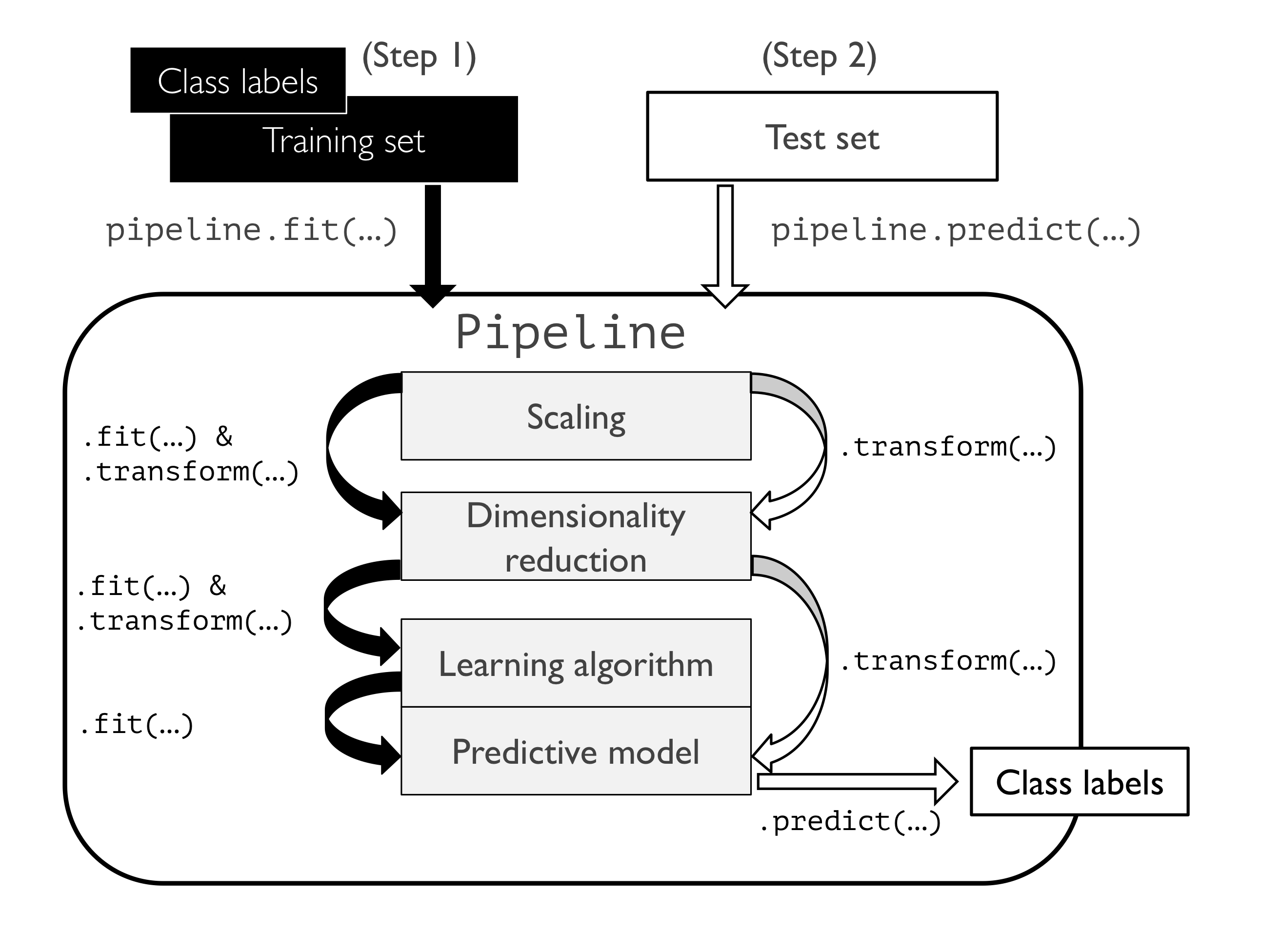
☑️StandardScaler, PCA, LogisticRegression 객체를 하나의 파이프라인으로 연결☑️
make_pipeline 함수 : 여러 개의 사이킷런 변환기와 그 뒤에 fit 메서드와 predict 메서드를 구현한 사이킷런 추정기를 연결 가능 -> 입력으로 받은 객체들을 사용하여 사이킷런의 Pipeline 클래스 객체를 생성하여 반환
from sklearn.preprocessing import StandardScaler
from sklearn.decomposition import PCA
from sklearn.linear_model import LogisticRegression
from sklearn.pipeline import make_pipeline

pipe_lr = make_pipeline(StandardScaler(),
                        PCA(n_components=2),
                        LogisticRegression(random_state=1))

pipe_lr.fit(X_train, y_train)
y_pred = pipe_lr.predict(X_test)
print('테스트 정확도: %.3f' % pipe_lr.score(X_test, y_test))
📍사이킷런의 파이프라인 작동 방식📍
6.2 k-겹 교차 검증을 사용한 모델 성능 평가
6.2.1 홀드아웃 방법
모델 선택 : 주어진 분류 문제에서 튜닝할 파라미터(하이퍼파라미터)의 최적 값을 선택해야 하는 것
📍홀드아웃 교차 검증📍
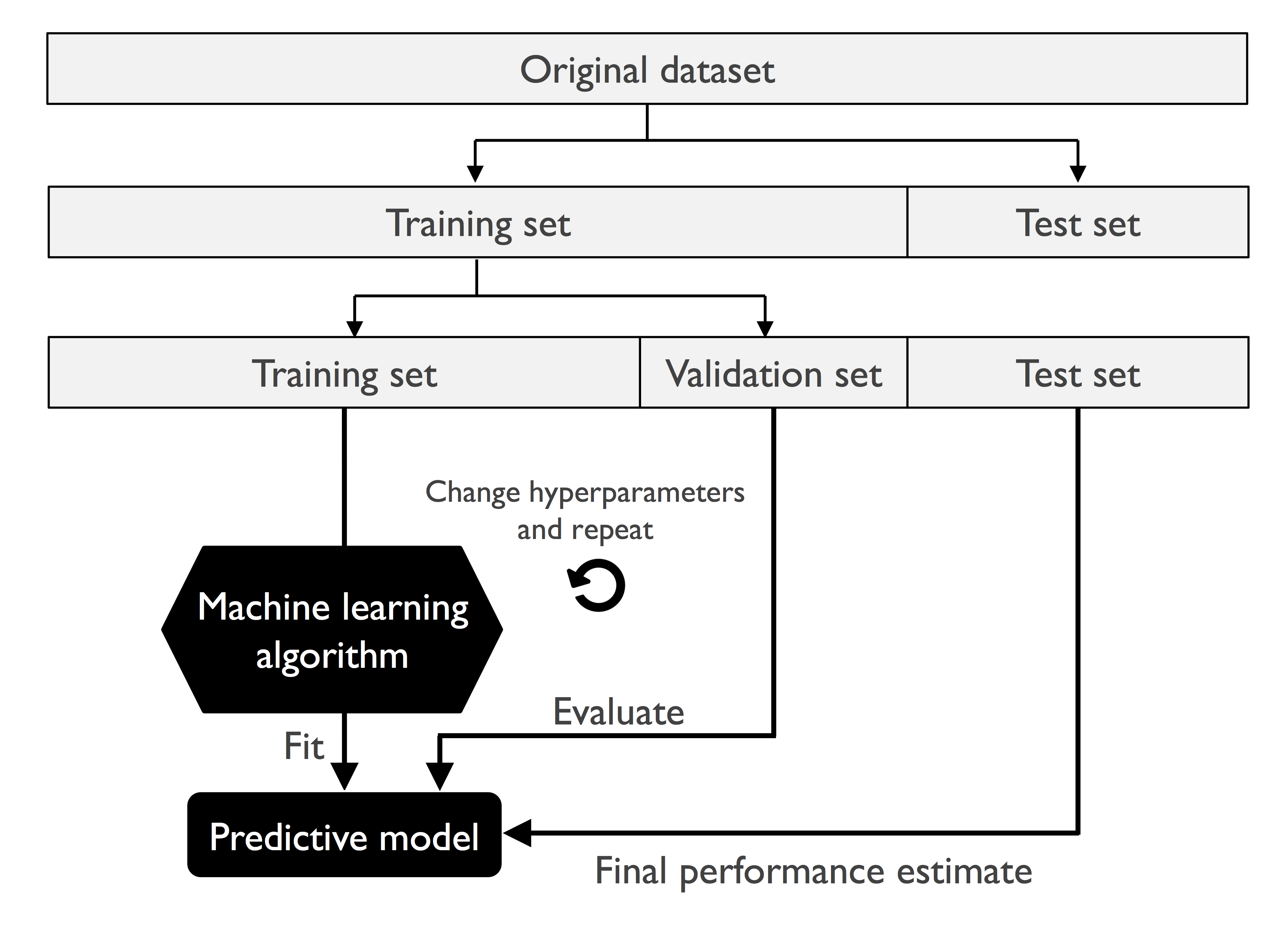
📍단점📍
검증 데이터셋의 성능 추정이 어떤 샘플을 사용하느냐에 따라 민감하게 달라짐
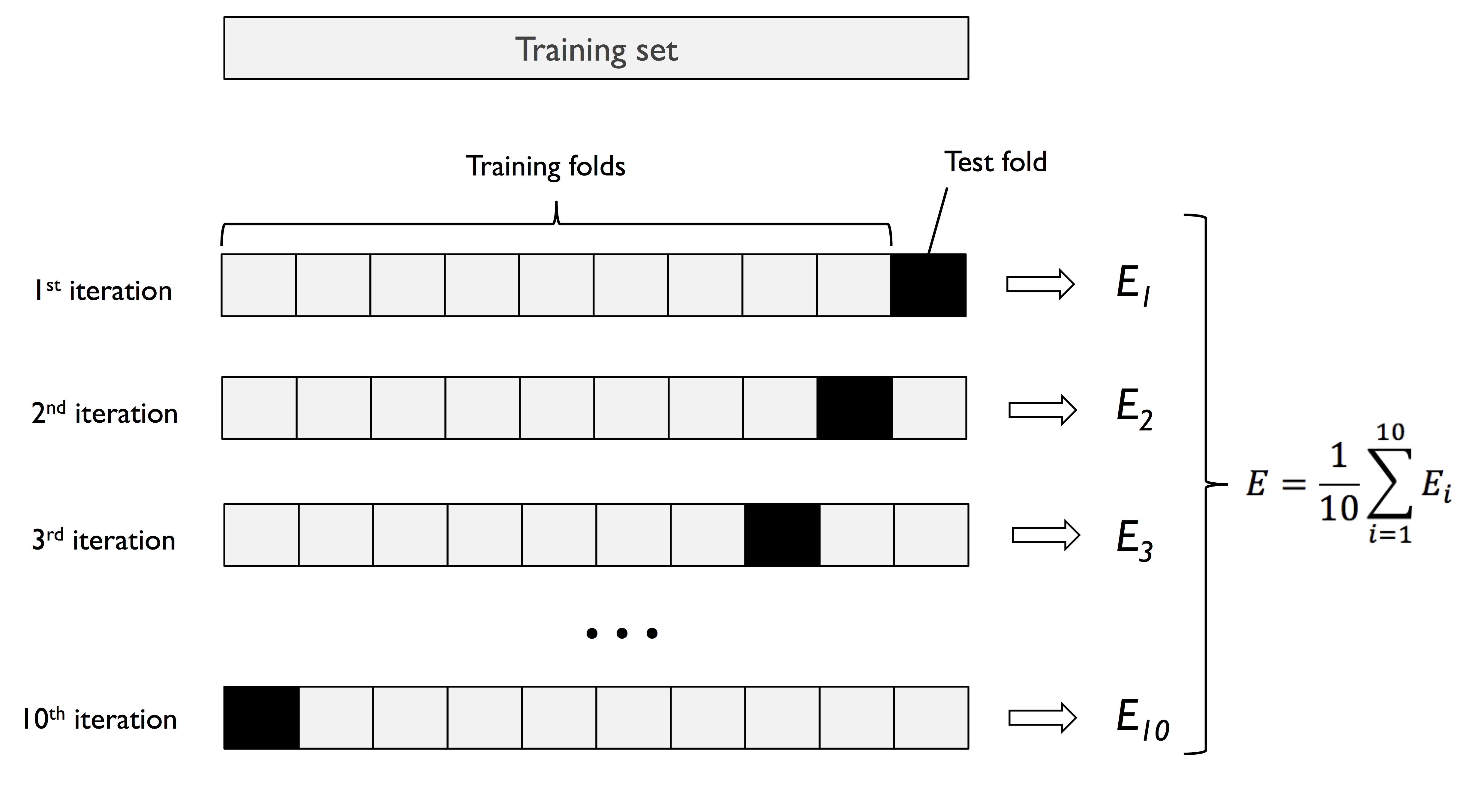
6.2.2 k-겹 교차 검증
k-겹 교차 검증 : 훈련 데이터를 k개의 부분으로 나누어 k번 홀드아웃 방법을 반복 / 훈련 데이터셋을 k개의 폴드로 랜덤하게 나눔 -> k-1개의 폴드로 모델을 훈련하고 나머지 하나의 폴드로 성능을 평가 -> 이 과정을 k번 반복하여 k개의 모델과 성능 추정을 얻음 -> 서로 다른 독립적인 폴드에서 얻은 성능 추정을 기반으로 모델의 평균 성능을 계산
☑️사이킷런의 StratifiedKFold 반복자를 사용☑️
import numpy as np
from sklearn.model_selection import StratifiedKFold

kfold = StratifiedKFold(n_splits=10).split(X_train, y_train)

scores = []
for k, (train, test) in enumerate(kfold):
    pipe_lr.fit(X_train[train], y_train[train])
    score = pipe_lr.score(X_train[test], y_train[test])
    scores.append(score)
    print('폴드: %2d, 클래스 분포: %s, 정확도: %.3f' % (k+1,
          np.bincount(y_train[train]), score))

print('\nCV 정확도: %.3f +/- %.3f' % (np.mean(scores), np.std(scores)))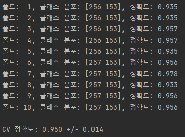
☑️사이킷런의 k-겹 교차 검증 함수 사용☑️
from sklearn.model_selection import cross_val_score

scores = cross_val_score(estimator=pipe_lr,
                         X=X_train,
                         y=y_train,
                         cv=10,
                         n_jobs=1)
print('CV 정확도 점수: %s' % scores)
print('CV 정확도: %.3f +/- %.3f' % (np.mean(scores), np.std(scores)))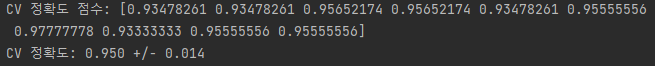
6.3 학습 곡선과 검증 곡선을 사용한 알고리즘 디버깅
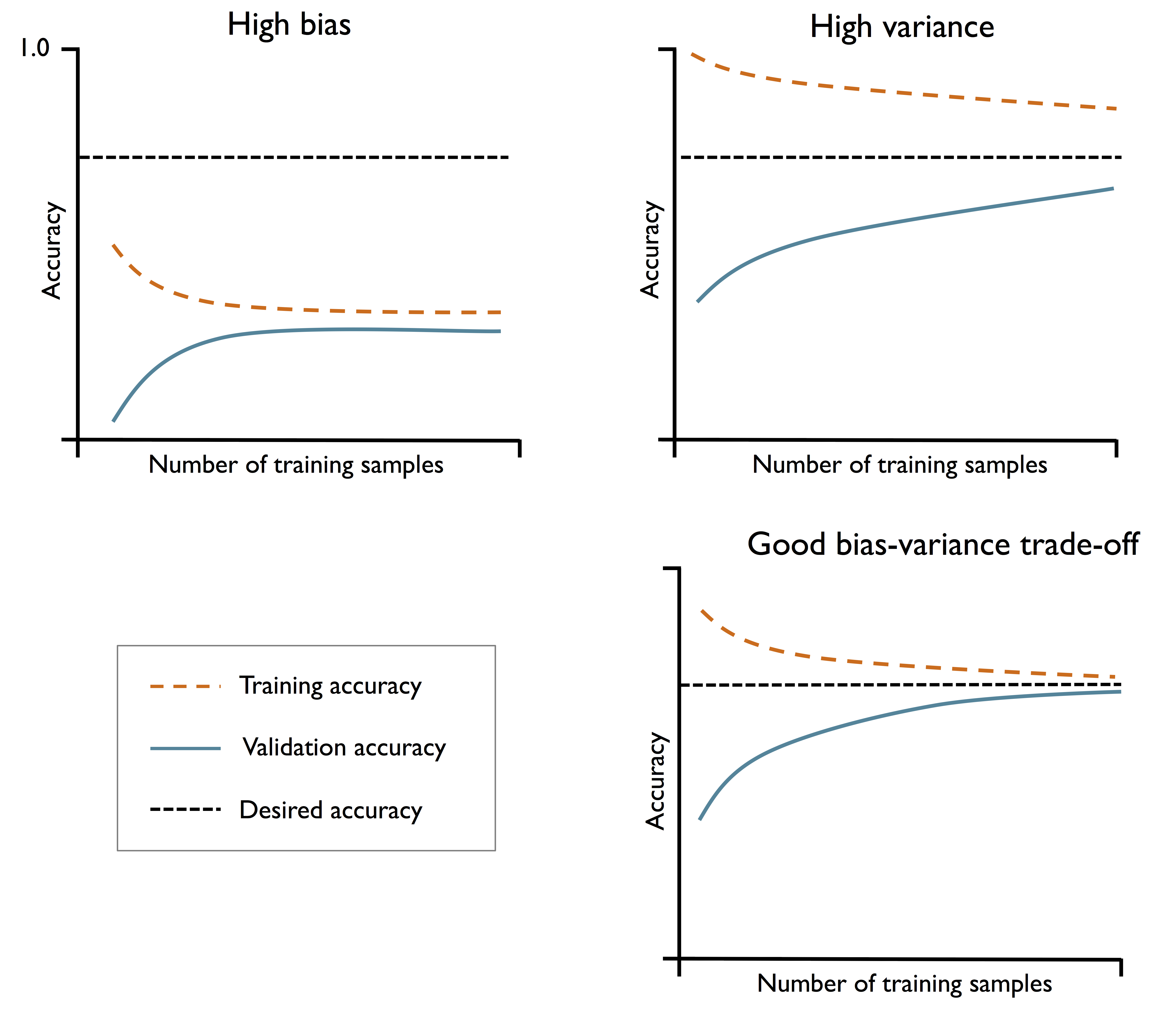
6.3.1 학습 곡선으로 편향과 분산 문제 분석
☑️사이킷런의 학습 곡선 함수를 사용하여 모델 평가☑️
- learning_curve 함수의 train_sizes 매개변수 : 학습 곡선을 생성하는 데 사용할 훈련 샘플의 개수나 비율을 지정
- learning_curve 함수 : 계층별 k-겹 교차 검증을 사용하여 분류기의 교차 검증 정확도를 계산
- fill_between 함수 : 그래프에 평균 정확도의 표준 편차를 그려서 추정 분산을 나타냄
import matplotlib.pyplot as plt
from sklearn.model_selection import learning_curve


pipe_lr = make_pipeline(StandardScaler(),
                        LogisticRegression(penalty='l2', random_state=1,
                                           max_iter=10000))

train_sizes, train_scores, test_scores =\
                learning_curve(estimator=pipe_lr,
                               X=X_train,
                               y=y_train,
                               train_sizes=np.linspace(0.1, 1.0, 10),
                               cv=10,
                               n_jobs=1)

train_mean = np.mean(train_scores, axis=1)
train_std = np.std(train_scores, axis=1)
test_mean = np.mean(test_scores, axis=1)
test_std = np.std(test_scores, axis=1)

plt.plot(train_sizes, train_mean,
         color='blue', marker='o',
         markersize=5, label='Training accuracy')

plt.fill_between(train_sizes,
                 train_mean + train_std,
                 train_mean - train_std,
                 alpha=0.15, color='blue')

plt.plot(train_sizes, test_mean,
         color='green', linestyle='--',
         marker='s', markersize=5,
         label='Validation accuracy')

plt.fill_between(train_sizes,
                 test_mean + test_std,
                 test_mean - test_std,
                 alpha=0.15, color='green')

plt.grid()
plt.xlabel('Number of training examples')
plt.ylabel('Accuracy')
plt.legend(loc='lower right')
plt.ylim([0.8, 1.03])
plt.tight_layout()
plt.show()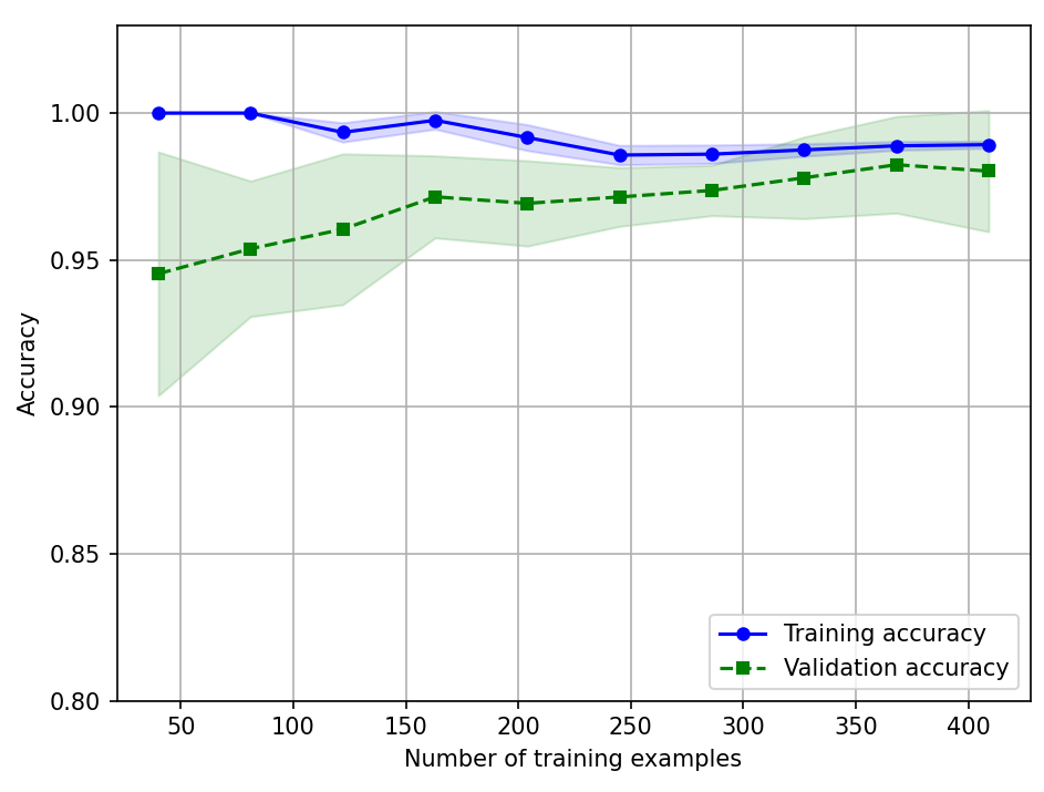
6.3.2 검증 곡선으로 과대적합과 과소적합 조사
☑️사이킷런으로 검증 곡선 만들기☑️
- validation_curv 함수 : 계층별 k-겹 교차 검증을 사용하여 모델의 성능을 추정
from sklearn.model_selection import validation_curve


param_range = [0.001, 0.01, 0.1, 1.0, 10.0, 100.0]
train_scores, test_scores = validation_curve(
                estimator=pipe_lr,
                X=X_train,
                y=y_train,
                param_name='logisticregression__C',
                param_range=param_range,
                cv=10)

train_mean = np.mean(train_scores, axis=1)
train_std = np.std(train_scores, axis=1)
test_mean = np.mean(test_scores, axis=1)
test_std = np.std(test_scores, axis=1)

plt.plot(param_range, train_mean,
         color='blue', marker='o',
         markersize=5, label='Training accuracy')

plt.fill_between(param_range, train_mean + train_std,
                 train_mean - train_std, alpha=0.15,
                 color='blue')

plt.plot(param_range, test_mean,
         color='green', linestyle='--',
         marker='s', markersize=5,
         label='Validation accuracy')

plt.fill_between(param_range,
                 test_mean + test_std,
                 test_mean - test_std,
                 alpha=0.15, color='green')

plt.grid()
plt.xscale('log')
plt.legend(loc='lower right')
plt.xlabel('Parameter C')
plt.ylabel('Accuracy')
plt.ylim([0.8, 1.0])
plt.tight_layout()
plt.show()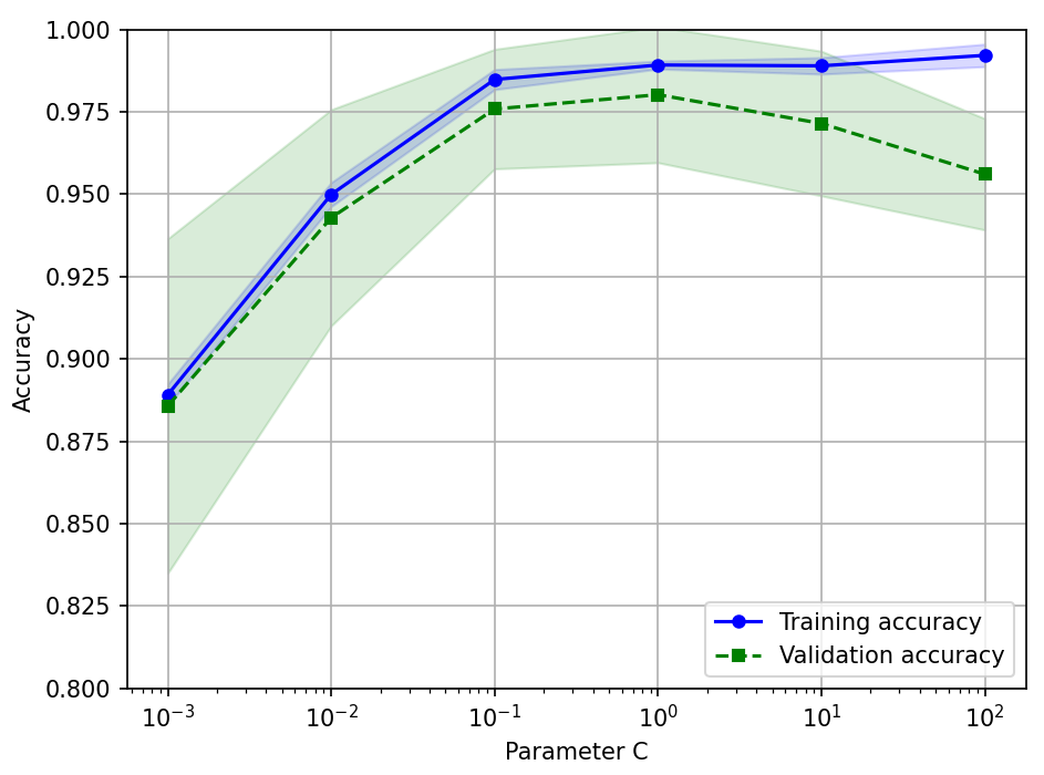
➡️매개변수 C에 대한 검증 곡선 그래프를 얻게 됨
6.4 그리드 서치를 사용한 머신 러닝 모델 세부 튜닝
튜닝 파라미터(하이퍼파라미터) : 별도로 최적화되는 학습 알고리즘의 파라미터
- 로지스틱 회귀의 규제 매개변수, 결정 트리의 깊이 매개변수
6.4.1 그리드 서치를 사용한 하이퍼파라미터 튜닝
그리드 서치 : 리스트로 지정된 여러 가지 하이퍼파라미터 값 전체를 모두 조사 -> 이 리스트에 있는 값의 모든 조합에 대해 모델 성능을 평가하여 최적의 조합을 찾음
☑️사이킷런 그리드 서치☑️
from sklearn.model_selection import GridSearchCV
from sklearn.svm import SVC

pipe_svc = make_pipeline(StandardScaler(),
                         SVC(random_state=1))

param_range = [0.0001, 0.001, 0.01, 0.1, 1.0, 10.0, 100.0, 1000.0]

param_grid = [{'svc__C': param_range,
               'svc__kernel': ['linear']},
              {'svc__C': param_range,
               'svc__gamma': param_range,
               'svc__kernel': ['rbf']}]

gs = GridSearchCV(estimator=pipe_svc,
                  param_grid=param_grid,
                  scoring='accuracy',
                  refit=True,
                  cv=10,
                  n_jobs=-1)
gs = gs.fit(X_train, y_train)
print(gs.best_score_)
print(gs.best_params_)
☑️독립적인 테스트 데이터셋을 사용하여 최고 모델의 성능을 추정☑️
clf = gs.best_estimator_

# refit=True로 지정했기 때문에 다시 fit() 메서드를 호출할 필요가 없습니다.
# clf.fit(X_train, y_train)

print('테스트 정확도: %.3f' % clf.score(X_test, y_test))
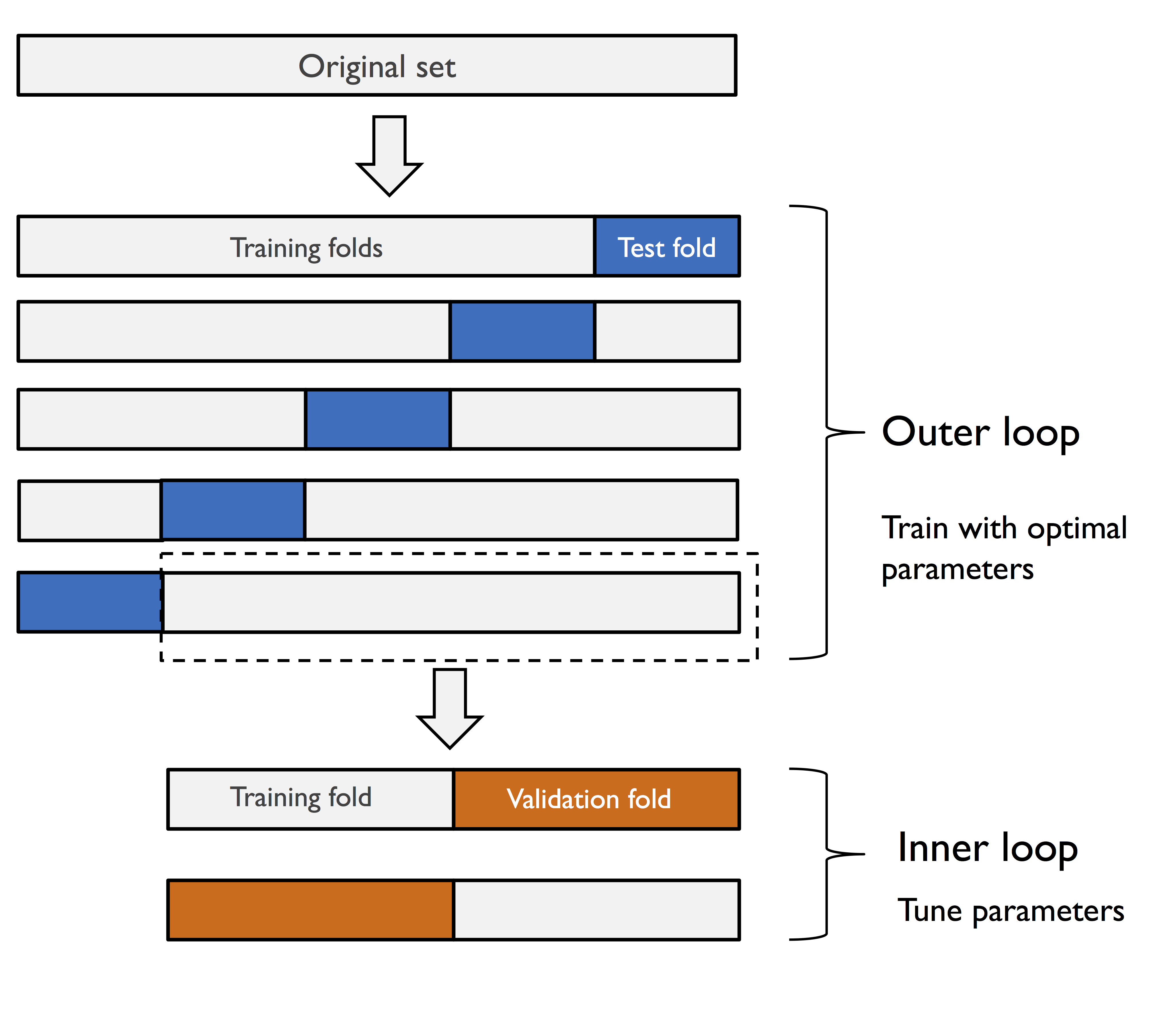
6.4.2 중첩 교차 검증을 사용한 알고리즘 선택
중첩 교차 검증 방법 - 여러 종류의 머신 러닝 알고리즘 비교할 때 권장
☑️사이킷런으로 중첩 교차 검증 수행☑️
gs = GridSearchCV(estimator=pipe_svc,
                  param_grid=param_grid,
                  scoring='accuracy',
                  cv=2)

scores = cross_val_score(gs, X_train, y_train,
                         scoring='accuracy', cv=5)
print('CV 정확도: %.3f +/- %.3f' % (np.mean(scores),
                                      np.std(scores)))
☑️max_depth 매개변수 튜닝☑️
from sklearn.tree import DecisionTreeClassifier

gs = GridSearchCV(estimator=DecisionTreeClassifier(random_state=0),
                  param_grid=[{'max_depth': [1, 2, 3, 4, 5, 6, 7, None]}],
                  scoring='accuracy',
                  cv=2)

scores = cross_val_score(gs, X_train, y_train,
                         scoring='accuracy', cv=5)
print('CV 정확도: %.3f +/- %.3f' % (np.mean(scores),
                                      np.std(scores)))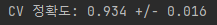
➡️ SVM 모델의 중첩 교차 검증 성능(97.4%)이 결정 트리의 성능(93.4%) 보다 훨씬 뛰어남
6.5 여러 가지 성능 평가 지표
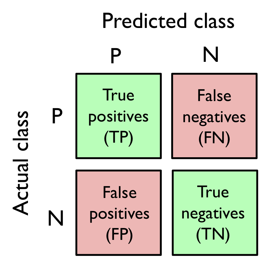
6.5.1 오차 행렬
☑️사이킷런 confusion_matrix 함수 사용☑️
from sklearn.metrics import confusion_matrix

pipe_svc.fit(X_train, y_train)
y_pred = pipe_svc.predict(X_test)
confmat = confusion_matrix(y_true=y_test, y_pred=y_pred)
print(confmat)
☑️오차 행렬 그리기☑️
matshow 함수 : 오차 행렬 그려줌
fig, ax = plt.subplots(figsize=(2.5, 2.5))
ax.matshow(confmat, cmap=plt.cm.Blues, alpha=0.3)
for i in range(confmat.shape[0]):
    for j in range(confmat.shape[1]):
        ax.text(x=j, y=i, s=confmat[i, j], va='center', ha='center')

plt.xlabel('Predicted label')
plt.ylabel('True label')

plt.tight_layout()
plt.show()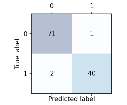
6.5.2 분류 모델의 정밀도와 재현율 최적화
오차 : 잘못된 예측의 합을 전체 예측 샘플 개수로 나눈 것
정확도 : 옳은 예측의 합을 전체 예측 샘플 개수로 나누어 계산
☑️사이킷런에서 성능 지표☑️
from sklearn.metrics import precision_score, recall_score, f1_score

print('정밀도: %.3f' % precision_score(y_true=y_test, y_pred=y_pred))
print('재현율: %.3f' % recall_score(y_true=y_test, y_pred=y_pred))
print('F1: %.3f' % f1_score(y_true=y_test, y_pred=y_pred))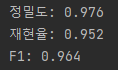
from sklearn.metrics import make_scorer

scorer = make_scorer(f1_score, pos_label=0)

c_gamma_range = [0.01, 0.1, 1.0, 10.0]

param_grid = [{'svc__C': c_gamma_range,
               'svc__kernel': ['linear']},
              {'svc__C': c_gamma_range,
               'svc__gamma': c_gamma_range,
               'svc__kernel': ['rbf']}]

gs = GridSearchCV(estimator=pipe_svc,
                  param_grid=param_grid,
                  scoring=scorer,
                  cv=10,
                  n_jobs=-1)
gs = gs.fit(X_train, y_train)
print(gs.best_score_)
print(gs.best_params_)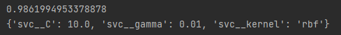
6.5.3 ROC 곡선 그리기
ROC 그래프 - 분류기의 임계 값을 바꾸어 가며 계산된 FPR과 TPR 점수를 기반으로 분류 모델을 선택하는 유용한 도구
☑️종양의 악성 여부를 예측하는 분류 모델의 ROC 곡선 그리기☑️
from sklearn.metrics import roc_curve, auc
from distutils.version import LooseVersion as Version
from scipy import __version__ as scipy_version


if scipy_version >= Version('1.4.1'):
    from numpy import interp
else:
    from scipy import interp


pipe_lr = make_pipeline(StandardScaler(),
                        PCA(n_components=2),
                        LogisticRegression(penalty='l2',
                                           random_state=1,
                                           C=100.0))

X_train2 = X_train[:, [4, 14]]


cv = list(StratifiedKFold(n_splits=3).split(X_train, y_train))

fig = plt.figure(figsize=(7, 5))

mean_tpr = 0.0
mean_fpr = np.linspace(0, 1, 100)

for i, (train, test) in enumerate(cv):
    probas = pipe_lr.fit(X_train2[train],
                         y_train[train]).predict_proba(X_train2[test])

    fpr, tpr, thresholds = roc_curve(y_train[test],
                                     probas[:, 1],
                                     pos_label=1)
    mean_tpr += interp(mean_fpr, fpr, tpr)
    mean_tpr[0] = 0.0
    roc_auc = auc(fpr, tpr)
    plt.plot(fpr,
             tpr,
             label='ROC fold %d (area = %0.2f)'
                   % (i+1, roc_auc))

plt.plot([0, 1],
         [0, 1],
         linestyle='--',
         color=(0.6, 0.6, 0.6),
         label='Random guessing')

mean_tpr /= len(cv)
mean_tpr[-1] = 1.0
mean_auc = auc(mean_fpr, mean_tpr)
plt.plot(mean_fpr, mean_tpr, 'k--',
         label='Mean ROC (area = %0.2f)' % mean_auc, lw=2)
plt.plot([0, 0, 1],
         [0, 1, 1],
         linestyle=':',
         color='black',
         label='Perfect performance')

plt.xlim([-0.05, 1.05])
plt.ylim([-0.05, 1.05])
plt.xlabel('False positive rate')
plt.ylabel('True positive rate')
plt.legend(loc="lower right")

plt.tight_layout()
plt.show()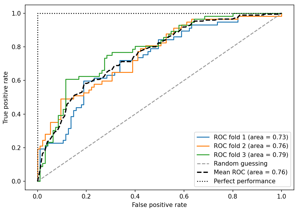
6.5.4 다중 분류의 성능 지표
pre_scorer = make_scorer(score_func=precision_score,
                         pos_label=1,
                         greater_is_better=True,
                         average='micro')
6.6 불균형한 클래스 다루기
☑️불균형한 유방암 데이터셋 만들기☑️
- 212개의 악성 종양(클래스 1)
- 357개의 양성 종양(클래스 0)
X_imb = np.vstack((X[y == 0], X[y == 1][:40]))
y_imb = np.hstack((y[y == 0], y[y == 1][:40]))
y_pred = np.zeros(y_imb.shape[0])
np.mean(y_pred == y_imb) * 100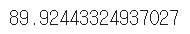
☑️사이킷런 소수 클래스의 샘플을 늘리기☑️
from sklearn.utils import resample

print('샘플링하기 전 클래스 1의 샘플 개수:', X_imb[y_imb == 1].shape[0])

X_upsampled, y_upsampled = resample(X_imb[y_imb == 1],
                                    y_imb[y_imb == 1],
                                    replace=True,
                                    n_samples=X_imb[y_imb == 0].shape[0],
                                    random_state=123)

print('샘플링하기 후 클래스 1의 샘플 개수:', X_upsampled.shape[0])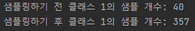
➡️데이터셋에서 다수 클래스의 훈련 샘플을 삭제하여 다운샘플링도 가능(클래스 레이블 1과 0을 서로 바꾸면 됨)

역시 대단해요~ 응원할게요! ^^