
개요
Databricks에서 ML을 하는 이유
| 항목 | 기존 ML 워크플로우 | Databricks 솔루션 |
|---|---|---|
| 환경 | 환경 불일치 (로컬 vs 서버 vs 프로덕션) | 통합 레이크하우스 (데이터 + ML + 서빙 한 플랫폼) |
| 실험 관리 | 실험 추적 부재 ("어떤 파라미터로 돌렸더라?") | Managed MLflow (자동 실험 추적 & 모델 버전 관리) |
| 재현성 | 재현 불가능 (과거 모델 재생성 어려움) | ML Runtime (사전 설치된 라이브러리 & GPU 지원) |
| 도구 구성 | 사일로화된 도구 (Jupyter + MLflow + Docker + K8s 등) | End-to-End 파이프라인 (AutoML → MLflow → Registry → Serving) |
- 예) 엔지니어, 사이언티스트, UI/UX들이 어디까지 본인이 작업할지 회의할 때, ML Flow를 기준으로 작업하자 하면 1분만에 끝남
엔지니어는 ML Flow에 저장, 사이언티스트, UI/UX는 ML Flow에서 읽기 Dev→Staging→Production단계- Production단계에선 실제 고객의 데이터 사용이 가능하지만, Dev에서도 일치시키긴 힘듦
- 따라서, 중간 단계인 Staging 단계를 마련하기도 함
- Spark는 1인 개발에 좋지만 협업은 힘들다
- 할거면 쿠버네티스에 올려서 사용
- Spark와 Databricks는 optimizer 기준으로 다르다.(Databricks가 더 빠름)
- Lake: 비정형 데이터까지 팍팍 넣겠음 / House: 웨어하우스(그 데이터를 꺼내 쓰겠다)
Databricks ML 컴포넌트 지도
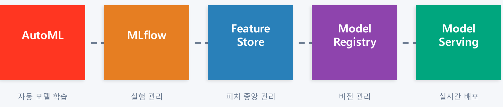
AutoML

- 생성된 소스 노트북을 읽고 커스터마이징 가능 → 투명성O (Explanable + Transparency)
- 10분 들여 설정해주면 알아서 모델을 완성해준다
- 사람은 최적 모델을 선택하기만 하면 됨
- photon 가속: photon은 c로 작성한 엔진으로 빠르다.
MLflow
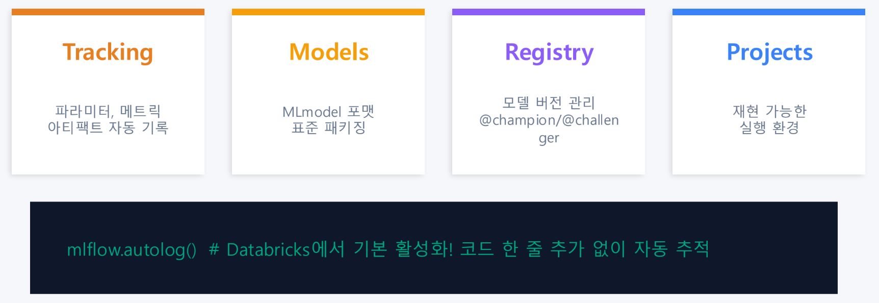
- 실험의 모든 것을 기록 가능
실습 1: Wine Quality 분류
분류 vs 회귀
- 분류: 범주가 불연속적(비 오냐 안오냐)
- 회귀: 범주가 연속적(비가 올 확률 60%)
Step 0: 환경 설정
import mlflow
import databricks.automl
Step 1: 데이터 로드 및 탐색
# Wine Quality 데이터셋 로드
from pyspark.sql import functions as F

# Databricks 내장 데이터셋 사용
white_wine = spark.read.csv(
    "dbfs:/databricks-datasets/wine-quality/winequality-white.csv", #dbfs: databricks file system
    header=True, #csv 파일 내에 헤더(컬럼명) 존재
    inferSchema=True, #정형/반정형 파일의 데이터 타입을 자동으로 추론
    sep=";" #구분자는 ;
)

# 컬럼명 정리 (공백 → 언더스코어)
for col_name in white_wine.columns:
    white_wine = white_wine.withColumnRenamed(col_name, col_name.replace(" ", "_"))

display(white_wine)- header false일 시, 첫 행부터 다 데이터로 인식
# 기본 통계 확인
display(white_wine.describe())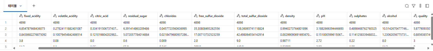
# 품질 분포 확인
display(white_wine.groupBy("quality").count().orderBy("quality"))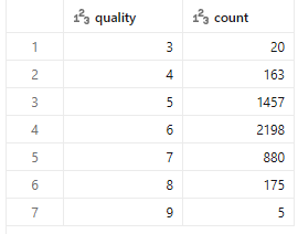
Step2: 이진 분류용 라벨 생성
품질 점수(3~9)를 좋음(1) / 보통(0) 이진 분류로 변환
# quality >= 7 이면 "좋은 와인"(1), 아니면 "보통"(0)
wine_df = white_wine.withColumn(
    "is_good_quality",
    F.when(F.col("quality") >= 7, 1).otherwise(0).cast("int")
)

# 라벨 분포 확인
display(wine_df.groupBy("is_good_quality").count())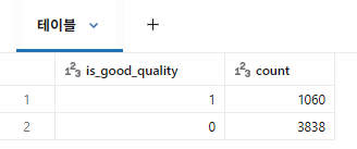
# Unity Catalog 테이블로 저장 (AutoML에서 사용)
# ⚠️ 카탈로그와 스키마를 수강생 환경에 맞게 수정하세요
CATALOG = "3dt016_databricks"
SCHEMA = "wine"
wine_df.write.mode("overwrite").saveAsTable(f"{CATALOG}.{SCHEMA}.wine_quality_lab")
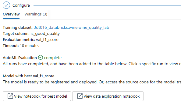
print(f"테이블 저장 완료: {CATALOG}.{SCHEMA}.wine_quality_lab")Step 3: AutoML 실행 — API 방식
Databricks 사용 방식
- UI 방식: Experiments 메뉴에서 클릭으로 실행
- API 방식: Python 코드로 실행
# AutoML 분류 실행
# 💡 timeout_minutes와 max_trials로 비용을 제어합니다
summary = databricks.automl.classify(
    dataset=f"{CATALOG}.{SCHEMA}.wine_quality_lab",
    target_col="is_good_quality",
    primary_metric="f1",
    timeout_minutes=10,  # 최대 10분
    max_trials=20,       # 최대 20개 모델 시도
    exclude_cols=["quality"],  # 원본 quality 컬럼 제외 (정보 누출 방지!)
)
1. 보고 싶은 모델 결과 선택
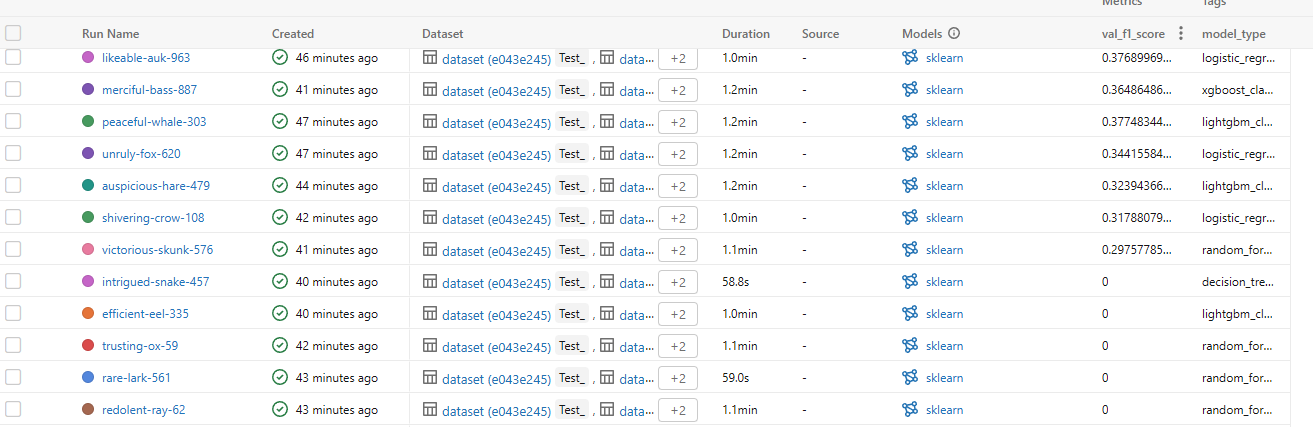
2. Arfifacts탭 선택 후 그래프 확인
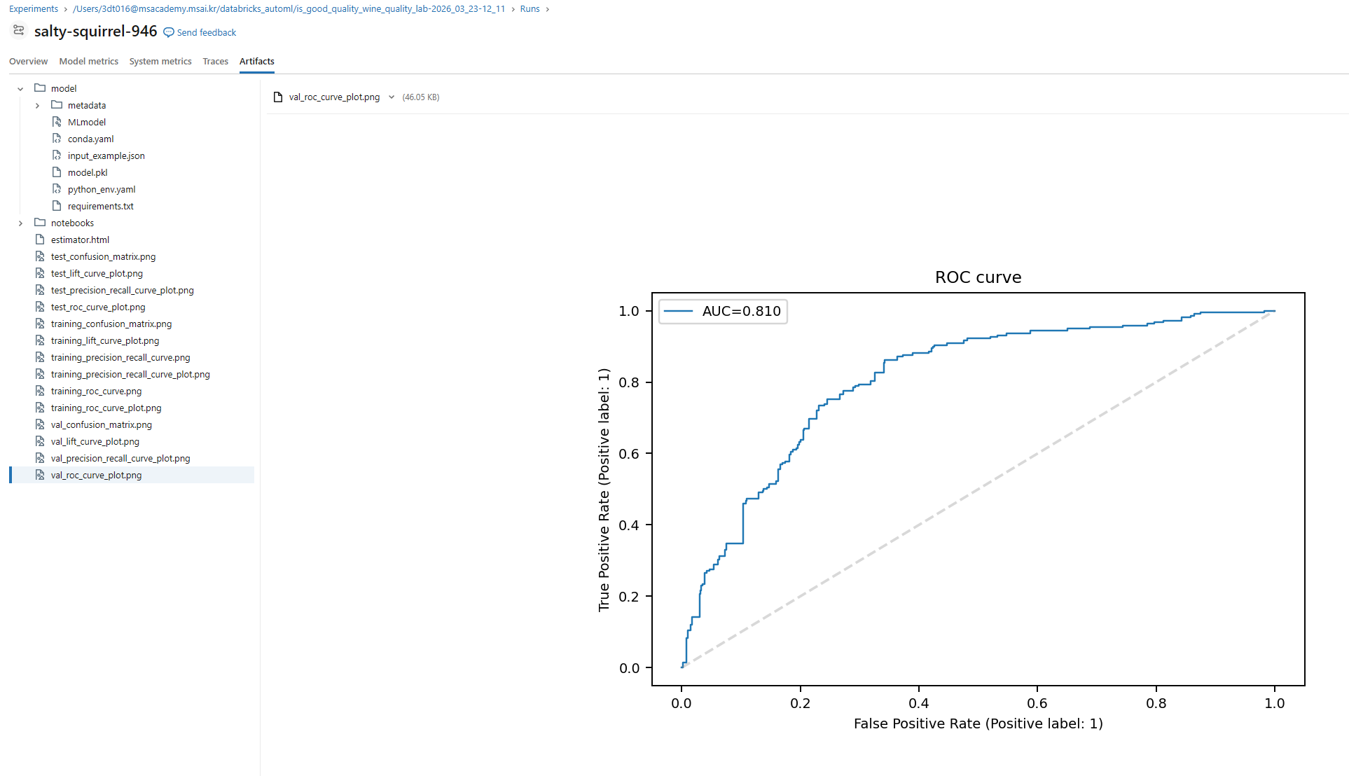
혹은 view best model 클릭 후 확인 가능
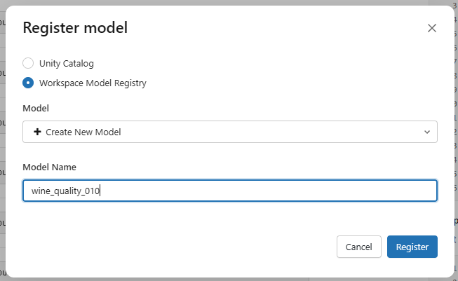
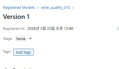
마음에 드는 모델은 우상단 Register Model 버튼으로 등록 가능
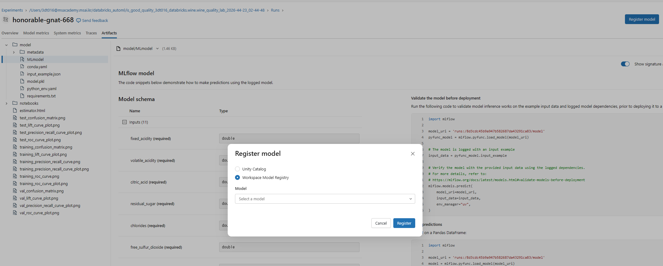
태그 추가 가능
사용하고자 하면 우상단 Use model for inference 선택
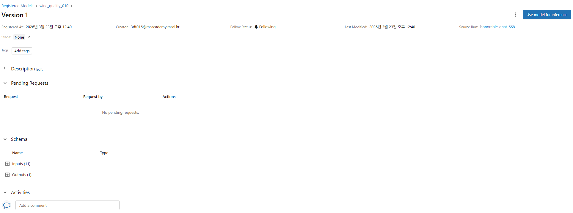
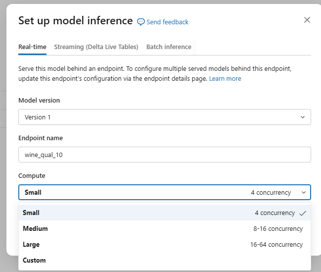
이렇게 해서 올리면 항상 호출 가능한 상태가 됨
이 엔드포인트를 사용해서 해당 모델 사용 가능(서빙)
이후 좌하단 서비스 탭에서 관리 가능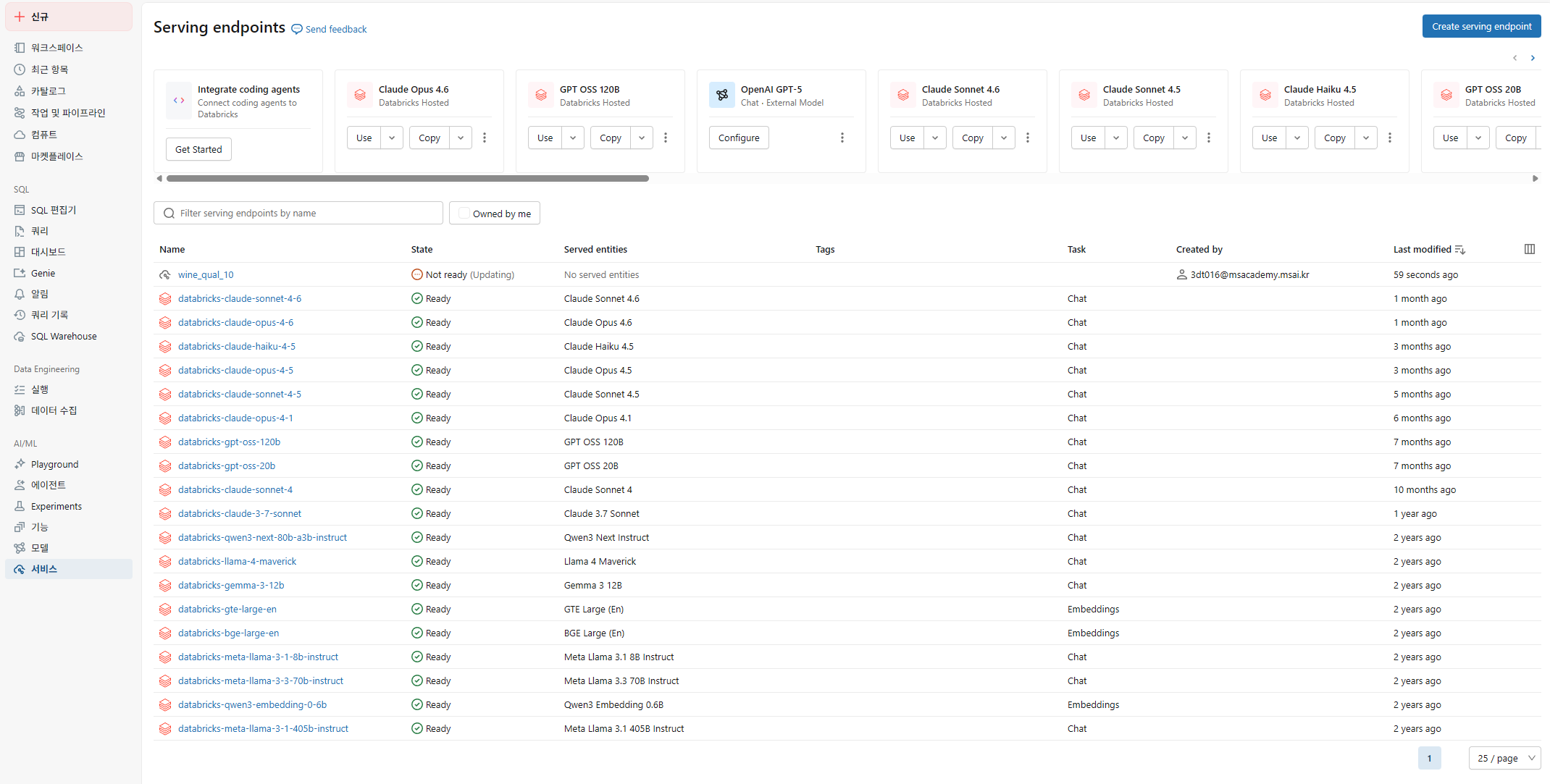
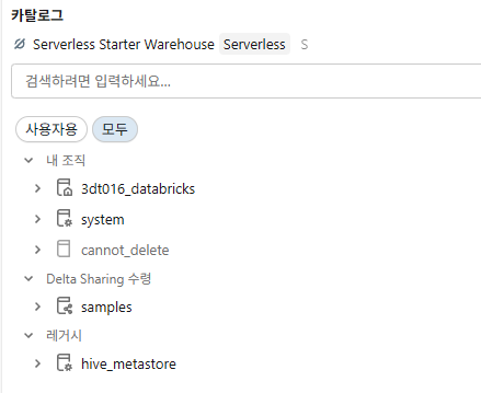
- legacy: hive_metastore는 예전에 사용했다(hadoob)
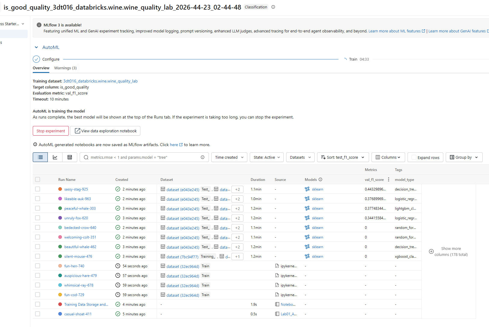
Step 3-2: AutoML UI 방식으로 실행
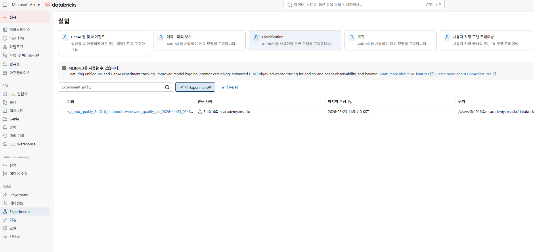
Experiments 탭 → Classification 선택
정답이 될 컬럼은 제외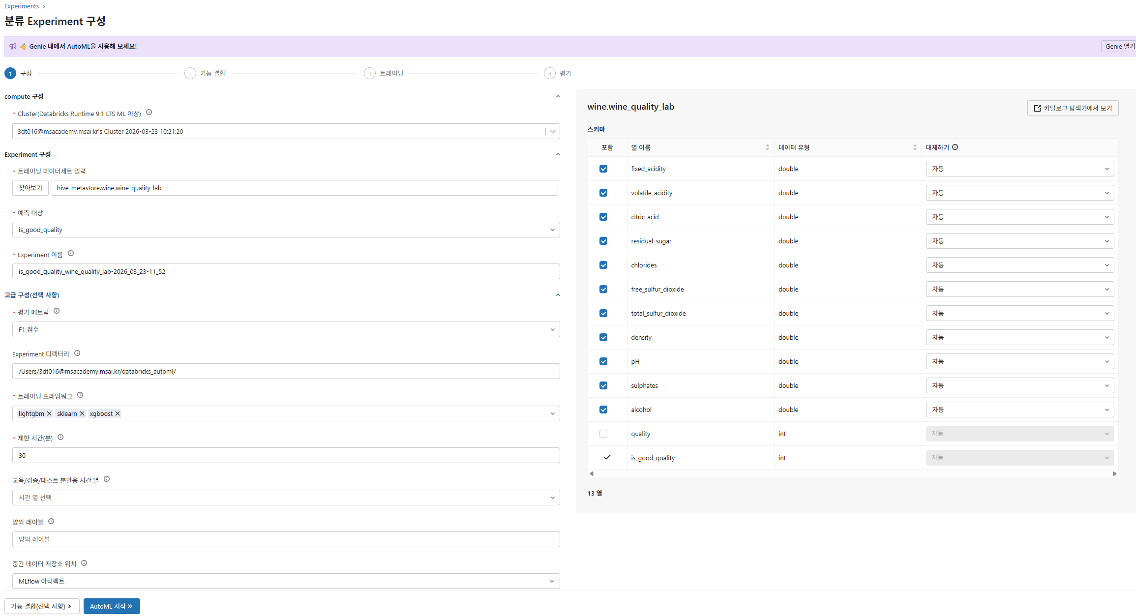
- 여기서 문제가 발생했는데, hive_metastore것이 아닌 기존 스키마의 것을 선택해줘야한다.
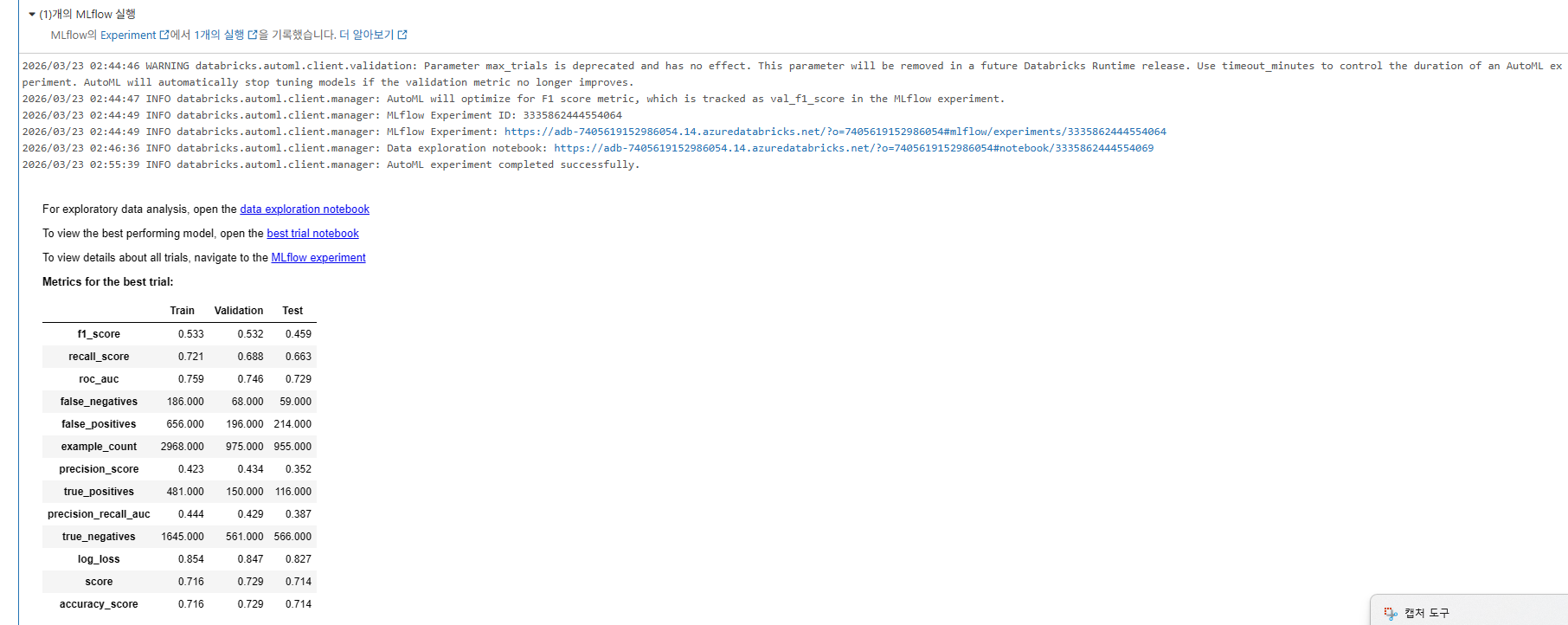
Step 4: AutoML 결과 분석
# 최적 모델 정보
print(f"🏆 최적 모델의 F1 Score: {summary.best_trial.metrics['test_f1_score']:.4f}")
print(f"📋 최적 모델 알고리즘: {summary.best_trial.model_description}")
print(f"🔗 MLflow Run ID: {summary.best_trial.mlflow_run_id}")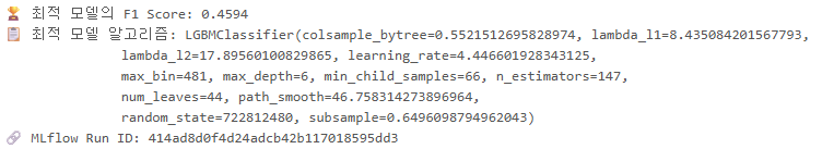
# 전체 실험 결과 확인
# 💡 Experiments UI에서 리더보드를 확인하면 더 직관적입니다!
print(f"\n총 {len(summary.trials)} 개 모델을 학습했습니다.")
print(f"실험 URL: {summary.experiment.experiment_id}")
print(f"\n📓 생성된 최적 노트북을 열어서 코드를 분석해보세요!")
print(f"노트북 URL: {summary.best_trial.notebook_url}")
# 최적 모델 로드 및 테스트
import mlflow
from sklearn.metrics import classification_report

best_model = mlflow.sklearn.load_model(f"runs:/{summary.best_trial.mlflow_run_id}/model")

# 테스트 데이터로 예측
test_pdf = wine_df.drop("quality").toPandas()
X_test = test_pdf.drop("is_good_quality", axis=1)
y_test = test_pdf["is_good_quality"]

y_pred = best_model.predict(X_test)
print(classification_report(y_test, y_pred, target_names=["보통", "좋음"]))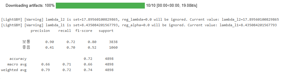
Step 5: SHAP Feature Importance 확인
import pandas as pd
import matplotlib.pyplot as plt

if hasattr(best_model, 'feature_importances_'):
    importance = pd.DataFrame({
        'feature': X_test.columns,
        'importance': best_model.feature_importances_
    }).sort_values('importance', ascending=True)

    fig, ax = plt.subplots(figsize=(10, 6))
    ax.barh(importance['feature'], importance['importance'], color='#FF3621')
    ax.set_title('Feature Importance — Wine Quality 분류')
    ax.set_xlabel('중요도')
    plt.tight_layout()
    display(fig)
else:
    print("이 모델은 feature_importances_ 속성이 없습니다. 노트북의 SHAP 분석을 참고하세요.")
핵심 정리
| 항목 | 내용 |
|---|---|
| AutoML 실행 | databricks.automl.classify() 한 줄이면 끝! |
| 자동화 범위 | 전처리 → 알고리즘 탐색 → 하이퍼파라미터 튜닝 → 교차 검증 |
| 투명성 | 생성된 소스 노트북을 열어서 코드를 읽고 수정 가능 |
| 비용 제어 | timeout_minutes와 max_trials로 실행 시간 제한 |
실습2: AutoML 회귀 — Airbnb 가격 예측
목표: 에어비앤비 숙소 특성으로 1박 가격을 예측하는 회귀 모델을 AutoML로 생성
Step 1: Airbnb 데이터 로드
from pyspark.sql import functions as F

# Databricks 내장 Airbnb 데이터셋 (San Francisco)
airbnb_df = spark.read.format("parquet").load(
    "dbfs:/databricks-datasets/learning-spark-v2/sf-airbnb/sf-airbnb-clean.parquet"
)

# 데이터 미리보기
print(f"총 {airbnb_df.count():,}개 숙소 데이터")
display(airbnb_df.limit(10))
parquet 사용 이유
- 높은 압축률
- 빠른 I/O
# 가격 분포 확인
display(airbnb_df.select("price").summary())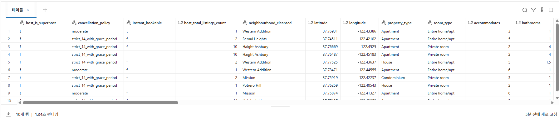
Step 2: 데이터 준비 & 테이블 저장
# 극단값 제거 (가격 $10~$1000)
airbnb_clean = airbnb_df.filter(
    (F.col("price") >= 10) & (F.col("price") <= 1000)
)

print(f"정제 후: {airbnb_clean.count():,}개 숙소")

# Unity Catalog 테이블로 저장
CATALOG = "3dt016_databricks"
SCHEMA = "airbnb"

airbnb_clean.write.mode("overwrite").saveAsTable(f"{CATALOG}.{SCHEMA}.airbnb_sf_lab")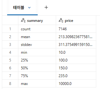
Step 3: AutoML 회귀 실행
import databricks.automl

# 💡 classify() 대신 regress()를 사용합니다!
summary = databricks.automl.regress(
    dataset=f"{CATALOG}.{SCHEMA}.airbnb_sf_lab",
    target_col="price",
    primary_metric="rmse",
    timeout_minutes=10,
    max_trials=20,
)
Step 4: 결과 분석
# 먼저 사용 가능한 메트릭 키 확인
print("📊 사용 가능한 메트릭 키:")
for k, v in sorted(summary.best_trial.metrics.items()):
    print(f"  {k}: {v}")

# 메트릭 키 자동 탐지 (AutoML 버전에 따라 키 이름이 다를 수 있음)
metrics = summary.best_trial.metrics
rmse_key = next((k for k in metrics if k in ("test_root_mean_squared_error", "test_rmse")), None)
r2_key = next((k for k in metrics if k in ("test_r2_score", "test_r2")), None)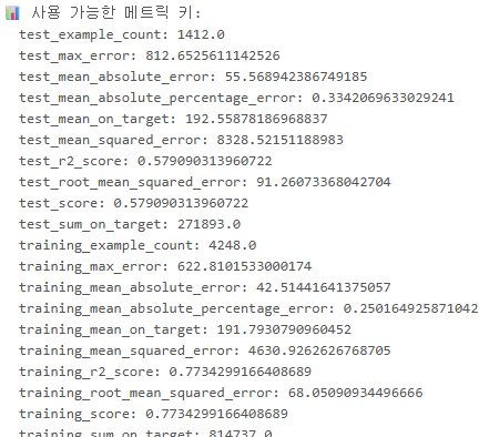
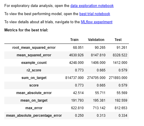
print(f"\n🏆 최적 모델 RMSE: {metrics[rmse_key]:.2f}" if rmse_key else "RMSE 키를 찾을 수 없음")
print(f"🏆 최적 모델 R²: {metrics[r2_key]:.4f}" if r2_key else "R² 키를 찾을 수 없음")
print(f"📋 알고리즘: {summary.best_trial.model_description}")
print(f"\n📓 생성된 노트북: {summary.best_trial.notebook_url}")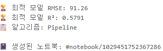
# 예측 vs 실제 가격 시각화
import mlflow
import matplotlib.pyplot as plt
import numpy as np

best_model = mlflow.sklearn.load_model(f"runs:/{summary.best_trial.mlflow_run_id}/model")

test_pdf = airbnb_clean.toPandas()
X_test = test_pdf.drop("price", axis=1)
y_test = test_pdf["price"]
y_pred = best_model.predict(X_test)

fig, ax = plt.subplots(figsize=(8, 8))
ax.scatter(y_test, y_pred, alpha=0.3, s=10, color='#FF3621')
ax.plot([0, 1000], [0, 1000], 'k--', alpha=0.5, label='Perfect Prediction')
ax.set_xlabel('Actual Price ($)', fontsize=12)
ax.set_ylabel('Predicted Price ($)', fontsize=12)
ax.set_title('Airbnb Price Prediction: Actual vs Predicted', fontsize=14)
ax.legend()
ax.set_xlim(0, 600)
ax.set_ylim(0, 600)
plt.tight_layout()
display(fig)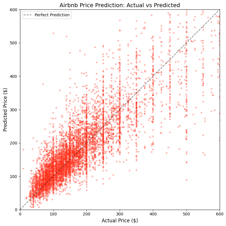
# Feature Importance
import pandas as pd

if hasattr(best_model, 'feature_importances_'):
    importance = pd.DataFrame({
        'feature': X_test.columns,
        'importance': best_model.feature_importances_
    }).sort_values('importance', ascending=False).head(10)

    fig, ax = plt.subplots(figsize=(10, 5))
    ax.barh(
        importance['feature'][::-1],
        importance['importance'][::-1],
        color='#00A67E'
    )
    ax.set_title('Top 10 Feature Importance — Airbnb 가격 예측')
    plt.tight_layout()
    display(fig)
# 모델 타입 확인
print(type(best_model))
print(hasattr(best_model, 'feature_importances_'))어떤 feature가 제일 중요한가 확인
# Feature Importance
# AutoML은 sklearn Pipeline으로 모델을 감싸므로, 내부 모델에 접근해야 합니다
import pandas as pd

# Pipeline 내부의 실제 모델 추출
if hasattr(best_model, 'named_steps'):
    final_model = list(best_model.named_steps.values())[-1]
elif hasattr(best_model, 'steps'):
    final_model = best_model.steps[-1][1]
else:
    final_model = best_model

print(f"Model type: {type(final_model)}")

if hasattr(final_model, 'feature_importances_'):
    # AutoML 전처리 후 피처 이름이 달라질 수 있으므로 모델에서 직접 가져옴
    # XGBoost/LightGBM 버전에 따라 피처 이름 속성이 다를 수 있음
    feature_names = None
    try:
        feature_names = final_model.get_booster().feature_names
    except Exception:
        pass
    if not feature_names:
        try:
            feature_names = list(final_model.feature_names_in_)
        except Exception:
            feature_names = [f"f{i}" for i in range(len(final_model.feature_importances_))]
    feature_names = [str(f) for f in feature_names]

    importance = pd.DataFrame({
        'feature': feature_names,
        'importance': final_model.feature_importances_.astype(float)
    }).sort_values('importance', ascending=False).head(10)

    fig, ax = plt.subplots(figsize=(10, 5))
    ax.barh(
        list(importance['feature'][::-1]),
        list(importance['importance'][::-1]),
        color='#00A67E'
    )
    ax.set_title('Top 10 Feature Importance — Airbnb Price')
    plt.tight_layout()
    display(fig)
else:
    print("This model doesn't expose feature_importances_ directly.")
    print("Check the AutoML-generated notebook for SHAP analysis.")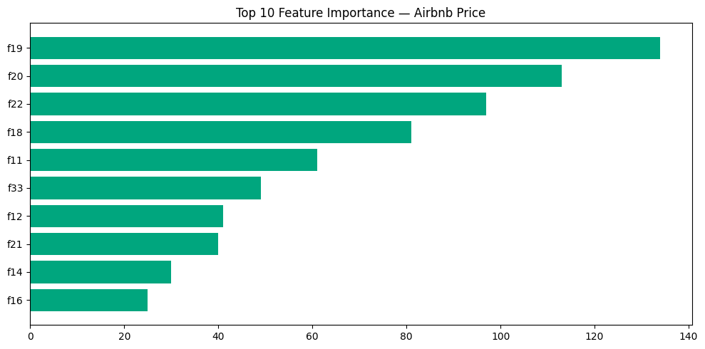
# AutoML이 생성한 노트북에서 피처 매핑 확인
print(f"원본 컬럼 수: {len(X_test.columns)}")
print(f"모델 피처 수: {len(final_model.feature_importances_)}")
print(f"\n원본 컬럼: {list(X_test.columns)}")
분류 vs 회귀 비교
| 항목 | 분류 (실습 1) | 회귀 (실습 2) |
|---|---|---|
| API | automl.classify() | automl.regress() |
| 타겟 | 이산값 (0/1) | 연속값 (가격) |
| 주요 메트릭 | F1, AUC, Accuracy | RMSE, MAE, R² |
| 시각화 | 혼동행렬, ROC | 예측 vs 실제 산점도 |
실습 3: AutoML 시계열 예측 — 매장 매출 예측
Part 1: 데이터 준비 — 리테일 매출 데이터 생성
- databricks.automl.forecast() API 사용법
- 시계열 데이터 전처리 (날짜 형식, 결측 처리)
- 단일/다중 시계열(multi-series) 예측
- Prophet & ARIMA 모델 결과 해석
- 예측 결과를 비즈니스 의사결정에 연결하기
import pandas as pd
import numpy as np
from pyspark.sql import functions as F
from pyspark.sql.types import *

np.random.seed(42)

# 2년간 일별 매출 데이터 생성 (3개 매장)
dates = pd.date_range("2023-01-01", "2025-02-28", freq="D")
stores = ["Seoul_Gangnam", "Seoul_Hongdae", "Busan_Haeundae"]

records = []
for store in stores:
    # 매장별 기본 매출 수준
    base_sales = {"Seoul_Gangnam": 5000, "Seoul_Hongdae": 3500, "Busan_Haeundae": 2800}
    base = base_sales[store]

    for date in dates:
        # 1) 연간 성장 트렌드 (연 10% 성장)
        years_from_start = (date - dates[0]).days / 365
        trend = base * (1 + 0.10 * years_from_start)

        # 2) 계절성 — 여름(7~8월) 피크, 겨울(1~2월) 저조
        month = date.month
        seasonality = {1: 0.75, 2: 0.78, 3: 0.90, 4: 0.95, 5: 1.05,
                       6: 1.10, 7: 1.25, 8: 1.20, 9: 1.05, 10: 0.95,
                       11: 1.00, 12: 1.15}  # 12월 연말 세일
        seasonal = trend * seasonality[month]

        # 3) 요일 효과 — 주말 매출 증가
        dow = date.dayofweek
        weekend_effect = 1.35 if dow >= 5 else 1.0  # 토/일 35% 증가
        friday_effect = 1.15 if dow == 4 else 1.0   # 금요일 15% 증가

        # 4) 특별 이벤트 (명절, 블랙프라이데이 등)
        special = 1.0
        if month == 1 and 20 <= date.day <= 25:  # 설날 연휴
            special = 1.5
        elif month == 9 and 15 <= date.day <= 20:  # 추석 연휴
            special = 1.4
        elif month == 11 and 24 <= date.day <= 27:  # 블랙프라이데이
            special = 1.8

        # 5) 랜덤 노이즈
        noise = np.random.normal(0, base * 0.08)

        daily_sales = max(0, seasonal * weekend_effect * friday_effect * special + noise)

        records.append({
            "date": date,
            "store_id": store,
            "daily_sales": round(daily_sales, 2),
            "day_of_week": date.strftime("%A"),
            "is_weekend": 1 if dow >= 5 else 0,
            "month": month,
        })

sales_pdf = pd.DataFrame(records)
sales_df = spark.createDataFrame(sales_pdf)

# Unity Catalog 테이블로 저장
CATALOG = "3dt016_databricks"   # ⚠️ 수강생 환경에 맞게 수정
SCHEMA = "forecasting"

sales_df.write.mode("overwrite").saveAsTable(f"{CATALOG}.{SCHEMA}.retail_sales_forecast")
print(f"✅ 데이터 저장 완료: {sales_df.count():,}건 ({len(stores)}개 매장 x {len(dates)}일)")
# 데이터 미리보기
display(spark.table(f"{CATALOG}.{SCHEMA}.retail_sales_forecast").orderBy("store_id", "date"))Part 2: 탐색적 분석 (EDA)
# 매장별 월간 매출 트렌드
monthly_sales = (
    spark.table(f"{CATALOG}.{SCHEMA}.retail_sales_forecast")
    .withColumn("year_month", F.date_format("date", "yyyy-MM"))
    .groupBy("store_id", "year_month")
    .agg(F.sum("daily_sales").alias("monthly_sales"))
    .orderBy("store_id", "year_month")
)

display(monthly_sales)
# 요일별 평균 매출
dow_sales = (
spark.table(f"{CATALOG}.{SCHEMA}.retail_sales_forecast")
.groupBy("store_id", "day_of_week")
.agg(F.avg("daily_sales").alias("avg_daily_sales"))
.orderBy("store_id", "avg_daily_sales")
)
display(dow_sales)Part 3: AutoML Forecasting 실행
databricks.automl.forecast()는 내부적으로 Prophet과 ARIMA 알고리즘을 사용
import databricks.automl
import mlflow
3-A: 단일 매장 예측 (Single Series)
# 강남점 데이터만 추출
gangnam_df = (
    spark.table(f"{CATALOG}.{SCHEMA}.retail_sales_forecast")
    .filter(F.col("store_id") == "Seoul_Gangnam")
    .select("date", "daily_sales")
)

gangnam_df.write.mode("overwrite").saveAsTable(f"{CATALOG}.{SCHEMA}.gangnam_sales_forecast")

print(f"강남점 데이터: {gangnam_df.count()}일")
display(gangnam_df.orderBy("date").tail(10))
# AutoML Forecasting 실행 — 단일 시계열
summary_single = databricks.automl.forecast(
dataset=f"{CATALOG}.{SCHEMA}.gangnam_sales_forecast",
target_col="daily_sales", # 예측할 컬럼
time_col="date", # 시간 컬럼
frequency="d", # 일별 데이터 (d=daily, W=weekly, M=monthly)
horizon=30, # 30일 후까지 예측
timeout_minutes=10, # 비용 제어
)# 결과 확인
print("📊 사용 가능한 메트릭:")
for k, v in sorted(summary_single.best_trial.metrics.items()):
print(f" {k}: {v}")
print(f"\n📋 Best model: {summary_single.best_trial.model_description}")
print(f"📓 Generated notebook: {summary_single.best_trial.notebook_url}")3-B: 다중 매장 예측 (Multi-Series)
# 전체 매장 데이터 (AutoML에 필요한 컬럼만 선택)
all_stores_df = (
    spark.table(f"{CATALOG}.{SCHEMA}.retail_sales_forecast")
    .select("date", "store_id", "daily_sales")
)

all_stores_df.write.mode("overwrite").saveAsTable(f"{CATALOG}.{SCHEMA}.all_stores_sales_forecast")
# AutoML Forecasting — 다중 시계열
summary_multi = databricks.automl.forecast(
dataset=f"{CATALOG}.{SCHEMA}.all_stores_sales_forecast",
target_col="daily_sales",
time_col="date",
identity_col=["store_id"], # 💡 매장별로 개별 모델 학습!
frequency="d",
horizon=30,
timeout_minutes=15,
)print("📊 Multi-series 메트릭:")
for k, v in sorted(summary_multi.best_trial.metrics.items()):
print(f" {k}: {v}")
print(f"\n📋 Best model: {summary_multi.best_trial.model_description}")Part 4: 예측 결과 분석 & 시각화
# 최적 모델로 30일 예측 생성
import mlflow

best_run_id = summary_multi.best_trial.mlflow_run_id
model = mlflow.pyfunc.load_model(f"runs:/{best_run_id}/model")

# 예측용 데이터 준비 (AutoML forecast 모델은 predict에 미래 날짜 DataFrame 필요)
# AutoML이 생성한 노트북에서 예측 코드를 참고하세요
print(f"✅ 모델 로드 완료: runs:/{best_run_id}/model")
print(f"📓 상세 예측 코드는 AutoML 생성 노트북을 참고하세요:")
print(f"   {summary_multi.best_trial.notebook_url}")
AutoML 생성 노트북 활용 가이드
AutoML이 자동 생성한 노트북에는 다음 포함:
1. 데이터 전처리 코드 — 결측 처리, 리샘플링 등
2. Prophet/ARIMA 모델 학습 코드 — 하이퍼파라미터 포함
3. 예측 결과 시각화 — 실제 vs 예측, 신뢰 구간
4. 잔차 분석 — 모델 성능 진단
# 간단한 예측 시각화 (학습 데이터의 마지막 90일 + 예측 비교)
import matplotlib.pyplot as plt

# 강남점 최근 데이터
recent_gangnam = (
    spark.table(f"{CATALOG}.{SCHEMA}.retail_sales_forecast")
    .filter(F.col("store_id") == "Seoul_Gangnam")
    .filter(F.col("date") >= "2025-01-01")
    .orderBy("date")
    .toPandas()
)

fig, ax = plt.subplots(figsize=(14, 5))
ax.plot(recent_gangnam["date"], recent_gangnam["daily_sales"],
        color="#FF3621", linewidth=1.5, label="Actual Sales")

# 7일 이동평균 트렌드 추가
recent_gangnam["ma7"] = recent_gangnam["daily_sales"].rolling(7).mean()
ax.plot(recent_gangnam["date"], recent_gangnam["ma7"],
        color="#00A67E", linewidth=2, label="7-day Moving Avg")

ax.set_title("Seoul Gangnam Store — Daily Sales (2025)", fontsize=14)
ax.set_xlabel("Date")
ax.set_ylabel("Daily Sales (KRW 10K)")
ax.legend()
ax.grid(True, alpha=0.3)
plt.tight_layout()
display(fig)
# 매장별 요약 통계
store_summary = (
spark.table(f"{CATALOG}.{SCHEMA}.retail_sales_forecast")
.groupBy("store_id")
.agg(
F.avg("daily_sales").alias("avg_daily_sales"),
F.stddev("daily_sales").alias("stddev_sales"),
F.min("daily_sales").alias("min_sales"),
F.max("daily_sales").alias("max_sales"),
F.sum("daily_sales").alias("total_sales"),
)
.orderBy(F.desc("total_sales"))
)
display(store_summary)Part 5: 비즈니스 인사이트 도출
인사이트 1: 월별 매출 패턴 → 재고 계획
# 월별 매장별 평균 매출 히트맵 데이터
monthly_pattern = (
    spark.table(f"{CATALOG}.{SCHEMA}.retail_sales_forecast")
    .groupBy("store_id", "month")
    .agg(F.avg("daily_sales").alias("avg_sales"))
    .orderBy("store_id", "month")
    .toPandas()
)

pivot_df = monthly_pattern.pivot(index="store_id", columns="month", values="avg_sales")

fig, ax = plt.subplots(figsize=(12, 4))
im = ax.imshow(pivot_df.values, cmap="YlOrRd", aspect="auto")
ax.set_xticks(range(12))
ax.set_xticklabels(["Jan", "Feb", "Mar", "Apr", "May", "Jun",
                     "Jul", "Aug", "Sep", "Oct", "Nov", "Dec"])
ax.set_yticks(range(len(stores)))
ax.set_yticklabels(pivot_df.index)
ax.set_title("Monthly Avg Sales Heatmap by Store")
plt.colorbar(im, ax=ax, label="Avg Daily Sales")

# 각 셀에 값 표시
for i in range(len(pivot_df.index)):
    for j in range(12):
        val = pivot_df.values[i, j]
        ax.text(j, i, f"{val:,.0f}", ha="center", va="center", fontsize=8,
                color="white" if val > pivot_df.values.mean() else "black")

plt.tight_layout()
display(fig)
인사이트 2: 요일별 매출 패턴 → 인력 배치
dow_pattern = (
    spark.table(f"{CATALOG}.{SCHEMA}.retail_sales_forecast")
    .groupBy("store_id", "day_of_week")
    .agg(F.avg("daily_sales").alias("avg_sales"))
    .toPandas()
)

dow_order = ["Monday", "Tuesday", "Wednesday", "Thursday", "Friday", "Saturday", "Sunday"]
dow_pattern["day_of_week"] = pd.Categorical(dow_pattern["day_of_week"], categories=dow_order, ordered=True)
dow_pattern = dow_pattern.sort_values("day_of_week")

fig, ax = plt.subplots(figsize=(10, 5))
for store in stores:
    store_data = dow_pattern[dow_pattern["store_id"] == store]
    ax.plot(store_data["day_of_week"], store_data["avg_sales"],
            marker="o", linewidth=2, label=store)

ax.set_title("Avg Daily Sales by Day of Week", fontsize=14)
ax.set_xlabel("Day of Week")
ax.set_ylabel("Avg Daily Sales")
ax.legend()
ax.grid(True, alpha=0.3)
plt.xticks(rotation=45)
plt.tight_layout()
display(fig)
인사이트 3: 성장률 분석 → 경영 보고
# 연도별 매장별 매출 비교
yearly = (
    spark.table(f"{CATALOG}.{SCHEMA}.retail_sales_forecast")
    .withColumn("year", F.year("date"))
    .groupBy("store_id", "year")
    .agg(F.sum("daily_sales").alias("annual_sales"))
    .orderBy("store_id", "year")
)

display(yearly)
# 전년 대비 성장률
yearly_pdf = yearly.toPandas()
for store in stores:
store_data = yearly_pdf[yearly_pdf["store_id"] == store].sort_values("year")
if len(store_data) >= 2:
sales_2023 = store_data[store_data["year"] == 2023]["annual_sales"].values[0]
sales_2024 = store_data[store_data["year"] == 2024]["annual_sales"].values[0]
growth = (sales_2024 - sales_2023) / sales_2023 * 100
print(f"{store}: 2023→2024 YoY Growth = {growth:.1f}%")Part 6: 실습 후 정리
# 임시 테이블 정리
spark.sql(f"DROP TABLE IF EXISTS {CATALOG}.{SCHEMA}.gangnam_sales_forecast")
spark.sql(f"DROP TABLE IF EXISTS {CATALOG}.{SCHEMA}.all_stores_sales_forecast")
# retail_sales_forecast는 다른 실습에서 재활용 가능하므로 유지
print("✅ 임시 테이블 정리 완료")
print(f"ℹ️ {CATALOG}.{SCHEMA}.retail_sales_forecast 테이블은 유지됩니다.")
🎯 핵심 정리
| 항목 | 내용 |
|---|---|
| API | databricks.automl.forecast() |
| 알고리즘 | Prophet, ARIMA (자동 선택) |
| 단일 시계열 | time_col + target_col |
| 다중 시계열 | identity_col로 그룹 지정 → 매장/제품별 개별 모델 |
| 주요 파라미터 | frequency (d/W/M), horizon (예측 기간) |
| 비용 제어 | timeout_minutes로 실행 시간 제한 |
실무 활용 포인트
- 재고 관리: 월별 매출 패턴 → 계절별 발주 계획
- 인력 배치: 요일별 매출 패턴 → 주말/평일 인력 최적화
- 경영 보고: 성장률 분석 + 향후 매출 예측 → 투자/확장 의사결정
- 프로모션 효과: 특별 이벤트 기간 매출 변화 → 마케팅 ROI 측정
classify / regress / forecast 비교
| classify | regress | forecast | |
|---|---|---|---|
| 문제 | 범주 예측 | 수치 예측 | 미래 수치 예측 |
| 예시 | 이탈 여부 | 집 가격 | 다음달 매출 |
| 알고리즘 | XGBoost, LightGBM, RF | XGBoost, LightGBM, RF | Prophet, ARIMA |
| 특수 파라미터 | - | - | frequency, horizon, identity_col |
Databricks LLM
Foundation Model API
DBRX, Llama 3, Mixtral 등
토큰당 과금 — 저비용 실습
AI Functions (SQL)
ai_query()로 SQL 안에서
LLM 호출 — 감성분석, 요약
Vector Search + RAG
사내 문서 기반 Q&A
소규모 작업
비용 관리 팁
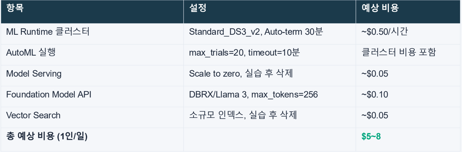
큰 머신 대신 작은 머신 여러개로 대체 가능한가? → 통신에 오버헤드가 발생하긴 함
vector search를 어떻게 저렴하게 하는가
- Foundation Model API는 토큰당 과금
- max_tokens 제한 설정
- 실습 후 리소스 삭제
- 1인당 $1 미만 목표
데이터사이언스 - 현업 예시
1. 데이터 사이언티스트의 현실과 실무 환경
- 실무 데이터 사이언티스트는 화려한 모델링보다 데이터 수집, 정제, 검증에 업무 시간의 60~80%를 할애함.
- 비즈니스 팀의 높은 기대치와 실제 데이터 품질 사이의 간극에서 발생하는 압박을 관리하며 문제를 해결하는 능력이 필수적임.
- 단순 반복적인 전처리나 코드 생성은 생성형 AI가 대체하고 있으며, 인간은 비즈니스 컨텍스트 이해와 전략적 판단에 더 집중해야 함.
2. 데이터 품질 문제와 기술적 해결 방안
데이터 품질은 모델의 성능을 결정하는 가장 중요한 요소이며, 이를 관리하기 위한 엔지니어링 역량이 요구됨.
- 주요 품질 문제: 센서 오류로 인한 결측치, 시스템 오류에 따른 중복 데이터, 측정 오류인 이상치, 시스템 통합 시 발생하는 데이터 불일치 및 수집 과정의 편향 문제.
- 데이터 프로파일링: 데이터 분포와 결측치 비율을 체계적으로 분석하여 상태를 객관적으로 파악함.
- 검증 자동화: Great Expectations, Pandera 등의 도구를 활용해 품질 검증 프로세스를 자동화하여 파이프라인의 안정성을 확보함.
- 모델 드리프트 대응: 배포 후 성능이 저하될 경우 데이터 분포 변화(Data Drift)인지 파악하고 최신 데이터로 신속히 재학습하는 MLOps 체계가 필요함.
3. 실무 사례별 핵심 역량
- 반도체 수율 예측: 기술적 정확도만큼 중요한 것이 설명 가능성임. SHAP나 LIME 등을 활용해 예측 근거를 시각화하여 이해관계자의 신뢰를 얻어야 함.
- 제조 라인 실시간 검사: 400ms 이내의 빠른 추론을 위해 MobileNet, EfficientNet과 같은 경량화 모델을 선택하고 엣지 컴퓨팅을 구축하는 능력이 요구됨.
- 식품 판매 예측: 제품 간 잠식 효과와 프로모션 영향을 분석하기 위해 다변량 시계열 모델(VAR)을 활용하며, 분석 결과를 ROI로 환산해 의사결정을 지원함.
4. 데이터 사이언티스트의 필수 스킬셋
- 엔지니어링 확장: Airflow, Spark를 활용한 ETL 파이프라인 설계 및 클라우드 기반 실시간 데이터 처리 역량.
- 비즈니스 가치 판단: 모델 정확도 1% 향상보다 그것이 실제 매출이나 비용 절감에 미치는 영향을 정량화하는 능력.
- 데이터 스토리텔링: 복잡한 지표에 내러티브를 더해 비전문가도 이해할 수 있도록 설득력 있게 전달하는 커뮤니케이션 기술.
5. 데이터 사이언티스트가 갖춰야 할 중요한 태도
데이터 사이언스의 핵심은 기술이 아닌 정직함에 있으며, 신뢰를 잃는 순간 분석의 가치도 사라짐.
- 단기 성과를 위해 데이터를 왜곡하지 않을 것: 의도적인 데이터 선택으로 결과를 조작하거나 자의적인 기준으로 이상치를 제거하는 행위를 지양해야 함.
- 불리한 결과를 숨기지 않을 것: 모델 성능이 낮거나 예측이 틀렸을 때 이를 투명하게 공유하고 실패 원인을 분석하여 조직의 학습 기회로 삼아야 함.
- 투명성의 원칙 준수: 데이터의 출처와 한계, 모델의 가정과 제약 사항을 명확히 공개하고 불확실성을 솔직하게 소통함.
- 윤리적 책임감: 상사의 데이터 조정 압박 등 윤리적 딜레마 상황에서도 정직한 태도를 유지하는 것이 장기적인 커리어 형성에 유리함.
6. 결론 및 성장 전략
- 기술 트렌드는 매년 변하지만 문제 해결 본질과 비즈니스 이해력은 영원한 가치를 지님.
- 완벽을 추구하기보다 빠르게 시도하고 배우며, 자신의 사고 과정이 담긴 포트폴리오를 GitHub나 블로그에 꾸준히 기록하는 것이 중요함.