[MicrosoftDataSchool] 57일차 - AzureDatabricks 추천 시스템(ALS), DeltaLake Table System, Pipeline

RudinP·2026년 3월 27일

AzureDatabricks MicrosoftDataSchool

Microsoft Data School 3기

목록 보기

48/68

협업 필터링	콘텐츠 기반 필터링
비슷한 취향을 가진 사용자들의 집단 행동 패턴을 분석합니다	아이템 자체의 특성과 메타데이터를 분석합니다
사용자 간 유사도 계산	장르, 키워드 매칭
평점 기반 예측	아이템 속성 분석
집단 지성 활용	프로필 기반 추천

구분	내용
장점	- 희소 데이터 처리 능력 우수 - 확장성이 뛰어나 대규모 서비스에 적합 - 과적합 방지 가능 - 오프라인 학습 후 빠른 추론
단점	- 모델 학습이 복잡하고 시간 소요 - 결과 해석이 어려움 - 하이퍼파라미터 튜닝 필요 - 신규 데이터 반영에 시간 지연

방법	설명
ε-그리디	ε 확률로 무작위 탐색, 1-ε 확률로 최선 선택
UCB	불확실성이 큰 선택지에 보너스를 부여하여 탐색
Thompson Sampling	베이지안 확률 분포에서 샘플링하여 선택

1. 실습 개요

기술 스택: Databricks, Spark MLlib, MLflow, Gradio
아키텍처: 메달리온 아키텍처 (Bronze → Silver → Gold)
핵심 알고리즘: ALS (Alternating Least Squares) 협업 필터링
데이터 규모: 영화 500개, 사용자 1,000명, 평점 약 10,000건 (희소성 약 98%)

2. 데이터 파이프라인 및 단계별 실습 내용

Step 1: 샘플 데이터 생성 (Bronze Layer)

실제 추천 시스템과 유사한 희소성(Sparsity)을 가진 가상의 영화, 사용자, 평점 데이터를 생성하여 Delta 테이블에 저장합니다.

주요 작업: 현실적인 평점 패턴(영화 품질 + 사용자 성향 + 노이즈)을 반영한 데이터 생성.
결과: 원시 데이터 형태의 bronze_movies, bronze_users, bronze_ratings 테이블 생성.

Step 2: 데이터 정제 및 피처 엔지니어링 (Silver Layer)

Bronze 데이터를 ML 모델 훈련에 적합한 형태로 변환합니다.

주요 변환: 장르 배열화, 연령대 인코딩, 태그 정규화 등.
핵심 개념 - 베이지안 평균(Bayesian Average): 평점 수가 적은 영화의 평점이 왜곡되는 것을 방지하기 위해 전체 평균과 최소 신뢰 샘플 수를 활용해 보정합니다.
- 공식: $bayesian\_avg = \frac{(v \times R + m \times C)}{(v + m)}$

Step 3: 모델 훈련 및 실험 추적 (Gold Layer & ML)

비즈니스 집계 데이터를 생성하고 ALS 모델을 최적화합니다.

ALS 알고리즘: 사용자-영화 행렬을 잠재 요인(Latent Factor)으로 분해하여 누락된 평점을 예측합니다.
MLflow 연동: 그리드 서치를 통해 rank, regParam 등의 하이퍼파라미터 조합을 실험하고, 모든 결과는 MLflow UI에 자동으로 기록 및 추적됩니다.

Step 4: 추천 서비스 구현

훈련된 모델을 활용하여 실제 추천 시나리오를 구성합니다.

추천 시나리오: 기존 사용자 추천, 장르 기반 추천, 유사 영화 탐색.
Cold Start 문제 해결: 평점 기록이 없는 신규 사용자를 위해 베이지안 평균 기반의 인기 영화를 추천하는 폴백(Fallback) 전략을 사용합니다.

Step 5: Gradio 인터랙티브 대시보드

사용자가 직접 추천 결과를 확인할 수 있는 웹 UI를 구축합니다.

주요 기능: 개인화 추천 ID 입력, 영화 제목 검색을 통한 유사 영화 탐색, 데이터 시각화 차트 등.

3. 핵심 개념 요약

용어	설명
메달리온 아키텍처	Bronze(원시) → Silver(정제) → Gold(집계) 순의 데이터 구조
ALS	협업 필터링을 위한 행렬 분해 알고리즘
Cold Start	신규 사용자/영화의 데이터 부족으로 인한 추천의 어려움
RMSE	예측 오차를 평가하는 지표 (낮을수록 정확함)
MLflow	머신러닝 실험 추적 및 모델 버전 관리 도구

4. 실습 후기 및 확장 과제

이번 실습을 통해 데이터 엔지니어링(메달리온 아키텍처)부터 모델 서빙(Gradio)까지의 전체 파이프라인을 경험할 수 있었습니다. 향후에는 다음과 같은 주제로 확장이 가능합니다.

Model Serving: REST API로 모델 배포
Feature Store: Databricks Feature Store 연동
Real-time: 실시간 스트리밍 데이터를 활용한 추천 반영

**콘텐츠 기반 필터링 결합**: 영화 메타데이터 기반 추천과 ALS 결합

샘플 영화 데이터 생성

영화 추천 시스템 실습을 위한 현실적인 샘플 데이터를 생성합니다.

생성할 데이터

테이블	설명	건수
movies	영화 메타데이터	500개
users	사용자 프로필	1,000명
ratings	사용자-영화 평점	~10,000건
tags	사용자 태그	1,000건

데이터 규모 설계 근거

실제 MovieLens Small 데이터셋 (ml-latest-small)은 약 600명 사용자, 9,000편 영화, 100,000건 평점 규모
본 실습에서는 학습·실행 시간을 고려하여 소규모로 설정
사용자당 평균 ~10개 평점 → 희소성(sparsity) 약 98% 수준 (현실적인 추천 시스템 환경)
사용자별 평점 수가 1~100개로 다양하게 분포 (실제 서비스와 유사한 롱테일 분포)

메달리온 아키텍처에서의 위치

이 노트북은 Bronze Layer (원시 데이터) 를 생성합니다.

[데이터 생성] → Bronze (원시) → Silver (정제) → Gold (집계/ML)
    ↑ 현재 위치

1. 환경 설정

Unity Catalog의 카탈로그와 스키마를 설정합니다.

CATALOG: 각자의 카탈로그 이름으로 변경하세요
SCHEMA: 이 실습에서 사용할 스키마 이름입니다

import pandas as pd
import numpy as np
from datetime import datetime, timedelta
import random
import json

# 재현성을 위한 시드 설정 (동일한 데이터를 반복 생성하기 위함)
np.random.seed(42)
random.seed(42)

# ============================================================
# ⚠️ 카탈로그 이름을 본인의 카탈로그로 변경하세요!
# ============================================================
CATALOG = "3dt016_databricks"
SCHEMA = "movie_recommender"

2. 스키마 생성

Unity Catalog 환경에서 데이터를 저장할 스키마(데이터베이스)를 생성합니다.
카탈로그는 이미 존재한다고 가정합니다. 없으면 CREATE CATALOG 주석을 해제하세요.

# 카탈로그가 없는 경우 아래 주석을 해제하세요
# spark.sql(f"CREATE CATALOG IF NOT EXISTS {CATALOG}")

# 스키마 생성 및 사용 설정
spark.sql(f"CREATE SCHEMA IF NOT EXISTS {CATALOG}.{SCHEMA}")
spark.sql(f"USE {CATALOG}.{SCHEMA}")

print(f"✅ 카탈로그/스키마 설정 완료: {CATALOG}.{SCHEMA}")

output

✅ 카탈로그/스키마 설정 완료: 3dt016_databricks.movie_recommender

3. 영화 데이터 생성

500개의 가상 영화 데이터를 생성합니다. 각 영화는 다음 속성을 가집니다:

movie_id: 고유 식별자 (1~500)
title: 영화 제목 (연도 포함)
year: 개봉 연도 (1970~2024, 최근 연도에 가중치)
genres: 장르 (1~4개, |로 구분)
director: 감독
runtime_minutes: 러닝타임
budget_millions: 예산 (백만 달러)
base_quality: 영화 품질 지표 (평점 생성 시 사용, 이후 제거됨)

# === 영화 메타데이터 정의 ===

# 18개 장르 (MovieLens 기준 표준 장르 분류)
GENRES = [
    "Action", "Adventure", "Animation", "Children", "Comedy", "Crime",
    "Documentary", "Drama", "Fantasy", "Film-Noir", "Horror", "Musical",
    "Mystery", "Romance", "Sci-Fi", "Thriller", "War", "Western"
]

# 유명 감독 목록 (다양한 국적 포함)
DIRECTORS = [
    "Christopher Nolan", "Steven Spielberg", "Martin Scorsese", "Quentin Tarantino",
    "Denis Villeneuve", "Ridley Scott", "James Cameron", "David Fincher",
    "Guillermo del Toro", "Peter Jackson", "Wes Anderson", "Coen Brothers",
    "Alfonso Cuarón", "Bong Joon-ho", "Park Chan-wook", "Wong Kar-wai",
    "Francis Ford Coppola", "Stanley Kubrick", "Alfred Hitchcock", "Akira Kurosawa"
]

# 영화 제목 생성을 위한 단어 사전
TITLE_PREFIXES = ["The", "A", "Return of", "Rise of", "Fall of", "Legend of", "Secret", "Last", "Dark", "Lost"]
TITLE_WORDS = [
    "Knight", "Dawn", "Storm", "Shadow", "Dragon", "Phoenix", "Empire", "Kingdom",
    "Warrior", "Journey", "Dream", "Destiny", "Heart", "Soul", "Fire", "Ice",
    "Thunder", "Ocean", "Mountain", "Forest", "City", "World", "Galaxy", "Universe"
]

def generate_movie_title():
    """
    랜덤 패턴을 사용하여 현실적인 영화 제목을 생성합니다.
    4가지 패턴: "The Knight", "Dawn of Storm", "Shadow: The Dragon", "Fire Ice"
    """
    pattern = random.choice([1, 2, 3, 4])
    if pattern == 1:
        return f"{random.choice(TITLE_PREFIXES)} {random.choice(TITLE_WORDS)}"
    elif pattern == 2:
        return f"{random.choice(TITLE_WORDS)} of {random.choice(TITLE_WORDS)}"
    elif pattern == 3:
        return f"{random.choice(TITLE_WORDS)}: {random.choice(TITLE_PREFIXES)} {random.choice(TITLE_WORDS)}"
    else:
        return f"{random.choice(TITLE_WORDS)} {random.choice(TITLE_WORDS)}"

def generate_movies(n_movies=500):
    """
    영화 데이터를 생성합니다.

    Args:
        n_movies: 생성할 영화 수 (기본값: 500)

    Returns:
        pd.DataFrame: 영화 메타데이터 DataFrame
    """
    movies = []
    used_titles = set()  # 제목 중복 방지

    for movie_id in range(1, n_movies + 1):
        # 고유한 제목 생성 (중복 시 재생성)
        while True:
            title = generate_movie_title()
            if title not in used_titles:
                used_titles.add(title)
                break

        # 연도: 삼각분포 사용 → 최근 연도에 더 많은 영화가 분포
        year = int(np.random.triangular(1970, 2010, 2024))

        # 장르: 1~4개 랜덤 할당
        n_genres = random.randint(1, 4)
        movie_genres = random.sample(GENRES, n_genres)

        director = random.choice(DIRECTORS)

        # 러닝타임: 정규분포 (평균 120분, 표준편차 25분), 75~210분 범위
        runtime = int(np.random.normal(120, 25))
        runtime = max(75, min(runtime, 210))

        # 예산: 지수분포 (대부분 저예산, 소수 블록버스터), 1~300M 범위
        budget = round(np.random.exponential(50), 1)
        budget = max(1, min(budget, 300))

        # 영화 품질 지표: Beta 분포 → 대부분 중간, 일부 고품질
        # Beta(5,3) * 3 + 2 = 2.0 ~ 5.0 분포
        base_rating = np.random.beta(5, 3) * 3 + 2

        movies.append({
            "movie_id": movie_id,
            "title": f"{title} ({year})",
            "year": year,
            "genres": "|".join(movie_genres),
            "director": director,
            "runtime_minutes": runtime,
            "budget_millions": budget,
            "base_quality": round(base_rating, 2)
        })

    return pd.DataFrame(movies)

# 영화 데이터 생성 실행
movies_df = generate_movies(500)
print(f"✅ 영화 데이터 생성 완료: {len(movies_df)}개")
movies_df.head(10)

output

✅ 영화 데이터 생성 완료: 500개

   movie_id                          title  ...  budget_millions base_quality
0         1            The Universe (1998)  ...              8.5         3.89
1         2               Lost Soul (1976)  ...            175.2         3.51
2         3      Kingdom of Thunder (1995)  ...             17.2         4.33
3         4            Kingdom Fire (2001)  ...             76.9         4.51
4         5   Dragon: Rise of Dream (2006)  ...              5.1         4.52
5         6       Legend of Destiny (1978)  ...            120.0         4.57
6         7            Dark Journey (2004)  ...            127.5         4.51
7         8   Storm: Rise of Shadow (2012)  ...             22.1         4.66
8         9  Empire: Fall of Galaxy (1982)  ...             65.3         4.24
9        10         Phoenix of Fire (2013)  ...             48.8         3.83

[10 rows x 8 columns]

4. 사용자 데이터 생성

500명의 가상 사용자를 생성합니다. 각 사용자는 다음 속성을 가집니다:

preference_profile: 장르 선호도 프로필 (7가지 유형) — 평점 생성 시 장르 매칭에 사용
activity_level: 활동성 (1~5) — 평점 개수 결정에 사용
rating_tendency: 평점 성향 (strict/neutral/lenient) — 평점 편향에 사용

이 속성들은 현실적인 평점 패턴을 만들기 위한 시뮬레이션 파라미터입니다.

# === 사용자 속성 정의 ===

COUNTRIES = ["USA", "UK", "Canada", "Germany", "France", "Japan", "Korea", "Australia", "Brazil", "India"]
AGE_GROUPS = ["18-24", "25-34", "35-44", "45-54", "55-64", "65+"]

# 장르 선호도 프로필: 사용자의 시청 취향을 모델링
# 각 프로필은 특정 장르에 대한 선호도 가중치(0~1)를 정의
GENRE_PREFERENCE_PROFILES = {
    "action_lover": {"Action": 0.9, "Adventure": 0.8, "Sci-Fi": 0.7, "Thriller": 0.6},
    "drama_enthusiast": {"Drama": 0.9, "Romance": 0.7, "Mystery": 0.6, "Film-Noir": 0.5},
    "comedy_fan": {"Comedy": 0.9, "Animation": 0.7, "Musical": 0.6, "Children": 0.5},
    "horror_seeker": {"Horror": 0.9, "Thriller": 0.8, "Mystery": 0.7, "Sci-Fi": 0.5},
    "family_viewer": {"Animation": 0.9, "Children": 0.8, "Comedy": 0.7, "Adventure": 0.6},
    "cinephile": {"Drama": 0.8, "Film-Noir": 0.8, "Documentary": 0.7, "War": 0.6},
    "balanced": {}  # 균형잡힌 취향 (특별한 선호 없음)
}

def generate_users(n_users=1000):
    """
    사용자 데이터를 생성합니다.

    Args:
        n_users: 생성할 사용자 수 (기본값: 1,000)

    Returns:
        pd.DataFrame: 사용자 프로필 DataFrame
    """
    users = []

    for user_id in range(1, n_users + 1):
        # 가입일: 2015~2024년 사이 랜덤
        days_since_start = random.randint(0, 365 * 9)
        signup_date = datetime(2015, 1, 1) + timedelta(days=days_since_start)

        country = random.choice(COUNTRIES)

        # 연령대: 25-34가 가장 많은 분포 (실제 스트리밍 서비스 인구통계 반영)
        age_weights = [0.15, 0.30, 0.25, 0.15, 0.10, 0.05]
        age_group = random.choices(AGE_GROUPS, weights=age_weights)[0]

        # 장르 선호도 프로필 랜덤 할당
        profile_type = random.choice(list(GENRE_PREFERENCE_PROFILES.keys()))

        # 활동성 레벨: 롱테일 분포 (다수 라이트 + 소수 헤비)
        activity_level = random.choices([1, 2, 3, 4, 5], weights=[0.20, 0.30, 0.30, 0.15, 0.05])[0]

        # 평점 성향: 대부분 neutral, 일부 strict(낮게 줌) 또는 lenient(높게 줌)
        rating_tendency = random.choice(["strict", "neutral", "neutral", "neutral", "lenient"])

        users.append({
            "user_id": user_id,
            "signup_date": signup_date.strftime("%Y-%m-%d"),
            "country": country,
            "age_group": age_group,
            "preference_profile": profile_type,
            "activity_level": activity_level,
            "rating_tendency": rating_tendency
        })

    return pd.DataFrame(users)

# 사용자 데이터 생성 실행
users_df = generate_users(1000)
print(f"✅ 사용자 데이터 생성 완료: {len(users_df)}명")
users_df.head(10)

output

✅ 사용자 데이터 생성 완료: 1000명

   user_id signup_date  ... activity_level rating_tendency
0        1  2020-02-05  ...              3         neutral
1        2  2023-01-11  ...              3          strict
2        3  2018-10-30  ...              2         lenient
3        4  2019-03-12  ...              2         neutral
4        5  2016-03-14  ...              1         neutral
5        6  2017-06-02  ...              3          strict
6        7  2023-06-29  ...              4         lenient
7        8  2016-05-19  ...              5         neutral
8        9  2020-08-05  ...              3         neutral
9       10  2021-07-24  ...              4         neutral

[10 rows x 7 columns]

5. 평점 데이터 생성 (핵심!)

평점 데이터는 추천 시스템의 핵심 입력입니다.

평점 계산 로직

각 평점은 다음 요소를 종합하여 현실적으로 생성됩니다:
1. 영화 품질 (base_quality): 기본 점수 (2.0~5.0)
2. 장르 매칭 보너스: 사용자 선호 장르와 일치하면 최대 +0.8점
3. 랜덤 노이즈: 정규분포 N(0, 0.5) — 개인차 반영
4. 평점 성향 보정: strict(-0.5), neutral(0), lenient(+0.5)
5. 최종 반올림: 0.5 단위, 0.5~5.0 범위

사용자별 평점 수 (롱테일 분포)

실제 서비스처럼 소수의 헤비 유저와 다수의 라이트 유저로 구성됩니다:
| 활동성 | 기본 평점 수 | 사용자 비율 |
|--------|-------------|-----------|
| 1 (낮음) | 1~3개 | 20% |
| 2 | 3~8개 | 30% |
| 3 (보통) | 8~15개 | 30% |
| 4 | 15~40개 | 15% |
| 5 (높음) | 40~100개 | 5% |

사용자당 평균 약 10개 평점 (총 ~10,000건 / 1,000명)

def calculate_rating(user, movie, genre_prefs):
    """
    사용자-영화 조합에 대한 현실적인 평점을 계산합니다.

    Args:
        user: 사용자 정보 딕셔너리
        movie: 영화 정보 딕셔너리
        genre_prefs: 사용자의 장르 선호도 딕셔너리

    Returns:
        float: 0.5 단위의 평점 (0.5 ~ 5.0)
    """
    # 1단계: 영화 자체의 품질이 기본 점수
    base = movie["base_quality"]

    # 2단계: 사용자 선호 장르와 영화 장르가 일치하면 보너스 부여
    movie_genres = set(movie["genres"].split("|"))
    genre_bonus = 0
    if genre_prefs:
        matching_prefs = [genre_prefs.get(g, 0) for g in movie_genres if g in genre_prefs]
        if matching_prefs:
            genre_bonus = np.mean(matching_prefs) * 0.8  # 최대 0.8점 보너스

    # 3단계: 랜덤 노이즈 (같은 영화라도 사용자마다 다르게 느낌)
    noise = np.random.normal(0, 0.5)

    # 4단계: 사용자 평점 성향 반영
    tendency_offset = {"strict": -0.5, "neutral": 0, "lenient": 0.5}
    tendency = tendency_offset.get(user["rating_tendency"], 0)

    # 최종 평점 계산 및 반올림
    rating = base + genre_bonus + noise + tendency
    rating = round(rating * 2) / 2  # 0.5 단위로 반올림
    rating = max(0.5, min(rating, 5.0))  # 범위 제한

    return rating

def generate_ratings(users_df, movies_df, target_ratings=10000):
    """
    평점 데이터를 생성합니다.

    각 사용자의 활동성 레벨에 비례하여 평점 수를 할당하고,
    영화 인기도(파레토 분포)에 따라 시청할 영화를 선택합니다.
    사용자별 평점 수는 롱테일 분포를 따릅니다 (소수 헤비유저 + 다수 라이트유저).

    Args:
        users_df: 사용자 DataFrame
        movies_df: 영화 DataFrame
        target_ratings: 목표 총 평점 수 (기본값: 10,000)

    Returns:
        pd.DataFrame: 평점 DataFrame
    """
    ratings = []

    users_list = users_df.to_dict("records")
    movies_list = movies_df.to_dict("records")

    # 영화 인기도: 파레토 분포 → 소수의 영화가 대부분의 평점을 받음 (롱테일 효과)
    movie_popularity = np.random.pareto(1.5, len(movies_list)) + 1
    movie_popularity = movie_popularity / movie_popularity.sum()

    # 사용자별 평점 수 결정 (활동성 기반, 롱테일 분포)
    # 실제 서비스와 유사하게: 대부분 적은 수, 소수가 많은 수
    user_rating_counts = []
    for user in users_list:
        activity = user["activity_level"]
        if activity == 1:
            # 라이트 유저: 1~3개
            count = random.randint(1, 3)
        elif activity == 2:
            # 가벼운 사용자: 3~8개
            count = random.randint(3, 8)
        elif activity == 3:
            # 보통 사용자: 8~15개
            count = random.randint(8, 15)
        elif activity == 4:
            # 활발한 사용자: 15~40개
            count = random.randint(15, 40)
        else:
            # 헤비 유저: 40~100개
            count = random.randint(40, 100)
        user_rating_counts.append(count)

    # 총 평점 수를 목표치에 맞게 스케일링
    total_planned = sum(user_rating_counts)
    scale_factor = target_ratings / total_planned
    user_rating_counts = [max(1, int(c * scale_factor)) for c in user_rating_counts]

    # 평점 생성
    for user, n_ratings in zip(users_list, user_rating_counts):
        # 사용자의 장르 선호도 가져오기
        genre_prefs = GENRE_PREFERENCE_PROFILES.get(user["preference_profile"], {})

        # 인기도 기반으로 시청할 영화 선택 (중복 없이, 영화 수 초과 방지)
        n_to_sample = min(n_ratings, len(movies_list))
        watched_indices = np.random.choice(
            len(movies_list),
            size=n_to_sample,
            replace=False,
            p=movie_popularity
        )

        # 평점 시간: 가입일 이후 랜덤 시점
        signup = datetime.strptime(user["signup_date"], "%Y-%m-%d")
        days_active = (datetime(2024, 12, 1) - signup).days

        for idx in watched_indices:
            movie = movies_list[idx]
            rating = calculate_rating(user, movie, genre_prefs)

            # 가입일 ~ 2024-12-01 사이의 랜덤 시점
            rating_days = random.randint(0, max(1, days_active))
            rating_time = signup + timedelta(
                days=rating_days,
                hours=random.randint(0, 23),
                minutes=random.randint(0, 59)
            )

            ratings.append({
                "user_id": user["user_id"],
                "movie_id": movie["movie_id"],
                "rating": rating,
                "timestamp": int(rating_time.timestamp())
            })

    return pd.DataFrame(ratings)

# 평점 데이터 생성 실행
print("⏳ 평점 데이터 생성 중...")
ratings_df = generate_ratings(users_df, movies_df, target_ratings=10000)
print(f"✅ 평점 데이터 생성 완료: {len(ratings_df):,}건")

# 평점 분포 확인
print("\n📊 평점 분포:")
print(ratings_df["rating"].value_counts().sort_index())

output

⏳ 평점 데이터 생성 중...
✅ 평점 데이터 생성 완료: 9,533건

📊 평점 분포:
1.5      21
2.0      82
2.5     317
3.0     852
3.5    1694
4.0    2210
4.5    2122
5.0    2235
Name: rating, dtype: int64

6. 태그 데이터 생성

사용자가 영화에 붙인 자유 태그 데이터를 생성합니다.

활발한 사용자(activity_level ≥ 3)만 태그를 작성한다고 가정
태그는 감성(긍정/부정/중립)을 포함하여 이후 분석에 활용 가능

# 영화 관련 태그 목록 (감성별 분류)
TAGS = [
    # 긍정적 태그
    "masterpiece", "must-watch", "amazing-visuals", "great-acting",
    "emotional", "inspiring", "beautiful", "rewatchable", "feel-good",
    # 부정적 태그
    "overrated", "boring", "predictable", "slow-paced",
    # 중립적/설명적 태그
    "underrated", "exciting", "thought-provoking", "mind-bending",
    "funny", "scary", "good-soundtrack", "twist-ending",
    "fast-paced", "complex-plot", "original", "classic", "cult-film",
    "dark", "violent", "family-friendly", "romantic", "disturbing", "nostalgic"
]

def generate_tags(users_df, movies_df, n_tags=1000):
    """
    태그 데이터를 생성합니다.

    Args:
        users_df: 사용자 DataFrame
        movies_df: 영화 DataFrame
        n_tags: 생성할 태그 수 (기본값: 1,000)

    Returns:
        pd.DataFrame: 태그 DataFrame
    """
    tags = []

    # 활발한 사용자만 태그 작성 (activity_level 3 이상)
    active_users = users_df[users_df["activity_level"] >= 3]["user_id"].tolist()

    for _ in range(n_tags):
        user_id = random.choice(active_users)
        movie_id = random.randint(1, len(movies_df))
        tag = random.choice(TAGS)

        # 태그 시간: 2020~2024년 사이 랜덤
        timestamp = int(datetime(2020, 1, 1).timestamp()) + random.randint(0, 157680000)

        tags.append({
            "user_id": user_id,
            "movie_id": movie_id,
            "tag": tag,
            "timestamp": timestamp
        })

    return pd.DataFrame(tags)

# 태그 데이터 생성 실행
tags_df = generate_tags(users_df, movies_df, n_tags=1000)
print(f"✅ 태그 데이터 생성 완료: {len(tags_df):,}건")

output

✅ 태그 데이터 생성 완료: 1,000건

7. Delta 테이블로 저장 (Bronze Layer)

생성된 데이터를 Delta Lake 형식의 Bronze 테이블로 저장합니다.

Bronze Layer는 원시 데이터를 그대로 보존하는 계층입니다:

데이터 변환 없이 원본 그대로 저장
overwrite 모드로 저장하여 재실행 시 기존 데이터를 덮어씁니다
Pandas DataFrame → Spark DataFrame → Delta Table 순으로 변환

from pyspark.sql.types import *

# Movies → Bronze 테이블
movies_spark = spark.createDataFrame(movies_df)
movies_spark.write.format("delta").mode("overwrite").saveAsTable(f"{CATALOG}.{SCHEMA}.bronze_movies")
print(f"✅ bronze_movies 테이블 저장 완료")

# Users → Bronze 테이블
users_spark = spark.createDataFrame(users_df)
users_spark.write.format("delta").mode("overwrite").saveAsTable(f"{CATALOG}.{SCHEMA}.bronze_users")
print(f"✅ bronze_users 테이블 저장 완료")

# Ratings → Bronze 테이블
ratings_spark = spark.createDataFrame(ratings_df)
ratings_spark.write.format("delta").mode("overwrite").saveAsTable(f"{CATALOG}.{SCHEMA}.bronze_ratings")
print(f"✅ bronze_ratings 테이블 저장 완료")

# Tags → Bronze 테이블
tags_spark = spark.createDataFrame(tags_df)
tags_spark.write.format("delta").mode("overwrite").saveAsTable(f"{CATALOG}.{SCHEMA}.bronze_tags")
print(f"✅ bronze_tags 테이블 저장 완료")

output

✅ bronze_movies 테이블 저장 완료
✅ bronze_users 테이블 저장 완료
✅ bronze_ratings 테이블 저장 완료
✅ bronze_tags 테이블 저장 완료

8. 데이터 요약

생성된 데이터의 통계를 확인합니다.
희소성(Sparsity) 은 전체 가능한 (사용자 × 영화) 조합 대비 실제 평점 비율의 여집합입니다.
희소성이 낮을수록(= 밀도가 높을수록) 협업 필터링 모델의 학습이 유리합니다.

print("=" * 60)
print("📊 생성된 데이터 요약")
print("=" * 60)
print(f"🎬 영화 수: {len(movies_df):,}개")
print(f"👤 사용자 수: {len(users_df):,}명")
print(f"⭐ 평점 수: {len(ratings_df):,}건")
print(f"🏷️  태그 수: {len(tags_df):,}건")
print(f"\n📍 저장 위치: {CATALOG}.{SCHEMA}")
print("=" * 60)

# 희소성(Sparsity) 계산
total_possible = len(movies_df) * len(users_df)  # 전체 가능한 조합
sparsity = 1 - (len(ratings_df) / total_possible)
print(f"\n🔢 평점 매트릭스 희소성: {sparsity:.4%}")
print(f"   (사용자당 평균 {len(ratings_df)/len(users_df):.1f}개 영화 평가)")
print(f"   (영화당 평균 {len(ratings_df)/len(movies_df):.1f}개 평점)")

output

============================================================
📊 생성된 데이터 요약
============================================================
🎬 영화 수: 500개
👤 사용자 수: 1,000명
⭐ 평점 수: 9,533건
🏷️  태그 수: 1,000건

📍 저장 위치: 3dt016_databricks.movie_recommender
============================================================

🔢 평점 매트릭스 희소성: 98.0934%
   (사용자당 평균 9.5개 영화 평가)
   (영화당 평균 19.1개 평점)

테이블	건수	설명
`bronze_movies`	500	영화 메타데이터
`bronze_users`	1,000	사용자 프로필
`bronze_ratings`	~10,000	사용자-영화 평점
`bronze_tags`	1,000	사용자 태그

Silver Layer: 데이터 정제 및 피처 엔지니어링

Bronze 데이터를 정제하고 ML에 활용할 수 있는 형태로 변환합니다.

변환 작업 요약

테이블	주요 변환
silver_movies	장르 배열화, 연대/예산/러닝타임 카테고리 생성, 정보 누출 컬럼 제거
silver_users	날짜 변환, 연령대 인코딩, 지역 그룹화, 평점 성향 수치화
silver_ratings	타임스탬프 변환, 시간대 카테고리, 평점 이진 레이블, 이상치 제거
silver_tags	태그 정규화, 감성 분류
silver_user_stats	사용자별 평점 통계 집계
silver_movie_stats	영화별 평점 통계 집계 + 베이지안 평균

메달리온 아키텍처에서의 위치

Bronze (원시) → Silver (정제/피처) → Gold (집계/ML)
                   ↑ 현재 위치

1. 환경 설정

from pyspark.sql import functions as F
from pyspark.sql.types import *
from pyspark.sql.window import Window
from datetime import datetime

# ============================================================
# ⚠️ 카탈로그 이름을 본인의 카탈로그로 변경하세요!
# ============================================================
CATALOG = "3dt016_databricks"
SCHEMA = "movie_recommender"

spark.sql(f"USE {CATALOG}.{SCHEMA}")
print(f"✅ 카탈로그 설정: {CATALOG}.{SCHEMA}")

output

✅ 카탈로그 설정: 3dt016_databricks.movie_recommender

2. Bronze 데이터 로드 및 탐색

이전 노트북에서 생성한 Bronze 테이블을 로드하고 기본 현황을 확인합니다.

# Bronze 테이블 로드
bronze_movies = spark.table("bronze_movies")
bronze_users = spark.table("bronze_users")
bronze_ratings = spark.table("bronze_ratings")
bronze_tags = spark.table("bronze_tags")

print("📊 Bronze 테이블 현황:")
print(f"  - movies:  {bronze_movies.count():,} rows")
print(f"  - users:   {bronze_users.count():,} rows")
print(f"  - ratings: {bronze_ratings.count():,} rows")
print(f"  - tags:    {bronze_tags.count():,} rows")

output

📊 Bronze 테이블 현황:
  - movies:  500 rows
  - users:   1,000 rows
  - ratings: 9,533 rows
  - tags:    1,000 rows

# 각 테이블의 샘플 데이터 확인
display(bronze_movies.limit(5))
display(bronze_users.limit(5))
display(bronze_ratings.limit(5))
display(bronze_tags.limit(5))

output

movie_id	title	year	genres	director	runtime_minutes	budget_millions	base_quality
1	The Universe (1998)	1998	Drama\|Western\|Comedy	Quentin Tarantino	92	8.5	3.89
2	Lost Soul (1976)	1976	Action	Martin Scorsese	145	175.2	3.51
3	Kingdom of Thunder (1995)	1995	Western	James Cameron	75	17.2	4.33
4	Kingdom Fire (2001)	2001	Action\|Crime\|Romance	Wes Anderson	101	76.9	4.51
5	Dragon: Rise of Dream (2006)	2006	Animation	Alfonso Cuarón	104	5.1	4.52

user_id	signup_date	country	age_group	preference_profile	activity_level	rating_tendency
1	2020-02-05	Japan	35-44	family_viewer	3	neutral
2	2023-01-11	Australia	18-24	balanced	3	strict
3	2018-10-30	Japan	45-54	balanced	2	lenient
4	2019-03-12	UK	18-24	drama_enthusiast	2	neutral
5	2016-03-14	France	35-44	drama_enthusiast	1	neutral

user_id	movie_id	rating	timestamp
1	479	4.0	1715870460
1	302	4.0	1605670560
1	351	4.0	1667179380
1	147	4.0	1732872300
1	195	5.0	1653249480

user_id	movie_id	tag	timestamp
426	425	must-watch	1619589428
374	212	mind-bending	1609074223
843	312	thought-provoking	1691535473
978	97	twist-ending	1595585111
796	434	romantic	1694484196

3. Silver Movies 변환

영화 데이터에 다음 피처를 추가합니다:

genres_array: 장르 문자열을 배열로 변환 (Explode 등 후속 분석에 필요)
num_genres: 장르 개수
decade: 연대 (1970, 1980, ...)
is_recent: 2015년 이후 영화 여부
budget_category: 예산 규모 카테고리 (Low/Medium/High/Blockbuster)
runtime_category: 러닝타임 카테고리 (Short/Standard/Long/Epic)

️ base_quality 컬럼 제거: 이 컬럼은 평점 생성용 시뮬레이션 파라미터이므로,
ML 모델 훈련 시 정보 누출(Data Leakage) 을 방지하기 위해 Silver 단계에서 삭제합니다.

silver_movies = (
    bronze_movies
    # 장르 문자열을 배열로 분리 (예: "Action|Comedy" → ["Action", "Comedy"])
    .withColumn("genres_array", F.split(F.col("genres"), "\\|"))
    .withColumn("num_genres", F.size("genres_array"))

    # 연도 기반 피처
    .withColumn("decade", (F.floor(F.col("year") / 10) * 10).cast("integer"))
    .withColumn("is_recent", F.when(F.col("year") >= 2015, True).otherwise(False))

    # 예산 카테고리 (백만 달러 기준)
    .withColumn("budget_category",
        F.when(F.col("budget_millions") < 20, "Low")        # 2천만 미만
        .when(F.col("budget_millions") < 80, "Medium")      # 2천만~8천만
        .when(F.col("budget_millions") < 150, "High")       # 8천만~1.5억
        .otherwise("Blockbuster")                            # 1.5억 이상
    )

    # 러닝타임 카테고리 (분 기준)
    .withColumn("runtime_category",
        F.when(F.col("runtime_minutes") < 90, "Short")      # 90분 미만
        .when(F.col("runtime_minutes") < 120, "Standard")   # 90~120분
        .when(F.col("runtime_minutes") < 150, "Long")       # 120~150분
        .otherwise("Epic")                                   # 150분 이상
    )

    # 처리 메타데이터
    .withColumn("processed_at", F.current_timestamp())
    .withColumn("data_quality_score", F.lit(1.0))

    # base_quality 제거 (정보 누출 방지)
    .drop("base_quality")
)

# 데이터 품질 검사: Null 값 확인
null_counts = silver_movies.select([
    F.sum(F.when(F.col(c).isNull(), 1).otherwise(0)).alias(c)
    for c in silver_movies.columns
])
print("🔍 Null 값 검사:")
null_counts.show()

# Silver 테이블 저장
silver_movies.write.format("delta").mode("overwrite").saveAsTable("silver_movies")
print(f"✅ silver_movies 저장 완료: {silver_movies.count():,} rows")

output

🔍 Null 값 검사:
+--------+-----+----+------+--------+---------------+---------------+------------+----------+------+---------+---------------+----------------+------------+------------------+
|movie_id|title|year|genres|director|runtime_minutes|budget_millions|genres_array|num_genres|decade|is_recent|budget_category|runtime_category|processed_at|data_quality_score|
+--------+-----+----+------+--------+---------------+---------------+------------+----------+------+---------+---------------+----------------+------------+------------------+
|       0|    0|   0|     0|       0|              0|              0|           0|         0|     0|        0|              0|               0|           0|                 0|
+--------+-----+----+------+--------+---------------+---------------+------------+----------+------+---------+---------------+----------------+------------+------------------+

✅ silver_movies 저장 완료: 500 rows

# 변환 결과 샘플 확인
display(silver_movies.limit(5))

output

movie_id	title	year	genres	director	runtime_minutes	budget_millions	genres_array	num_genres	decade	is_recent	budget_category	runtime_category	processed_at	data_quality_score
1	The Universe (1998)	1998	Drama\|Western\|Comedy	Quentin Tarantino	92	8.5	['Drama', 'Western', 'Comedy']	3	1990	False	Low	Standard	2026-03-27T01:35:12.904Z	1.0
2	Lost Soul (1976)	1976	Action	Martin Scorsese	145	175.2	['Action']	1	1970	False	Blockbuster	Long	2026-03-27T01:35:12.904Z	1.0
3	Kingdom of Thunder (1995)	1995	Western	James Cameron	75	17.2	['Western']	1	1990	False	Low	Short	2026-03-27T01:35:12.904Z	1.0
4	Kingdom Fire (2001)	2001	Action\|Crime\|Romance	Wes Anderson	101	76.9	['Action', 'Crime', 'Romance']	3	2000	False	Medium	Standard	2026-03-27T01:35:12.904Z	1.0
5	Dragon: Rise of Dream (2006)	2006	Animation	Alfonso Cuarón	104	5.1	['Animation']	1	2000	False	Low	Standard	2026-03-27T01:35:12.904Z	1.0

4. Silver Users 변환

사용자 데이터에 ML과 분석에 유용한 피처를 추가합니다:

날짜 관련: signup_date 타입 변환, 가입 연도/월, 계정 나이 (일수)
인코딩: 연령대 숫자 인코딩 (ML 입력용)
지역 그룹: 국가를 대륙/지역으로 그룹화
성향 수치화: 평점 성향을 -1/0/+1 수치로 변환

silver_users = (
    bronze_users
    # 날짜 타입 변환 (문자열 → Date)
    .withColumn("signup_date", F.to_date("signup_date"))
    .withColumn("signup_year", F.year("signup_date"))
    .withColumn("signup_month", F.month("signup_date"))

    # 가입 기간 계산 (오늘 기준)
    .withColumn("account_age_days",
        F.datediff(F.current_date(), F.col("signup_date"))
    )

    # 연령대 → 숫자 인코딩 (ML 모델 입력용)
    .withColumn("age_group_encoded",
        F.when(F.col("age_group") == "18-24", 1)
        .when(F.col("age_group") == "25-34", 2)
        .when(F.col("age_group") == "35-44", 3)
        .when(F.col("age_group") == "45-54", 4)
        .when(F.col("age_group") == "55-64", 5)
        .otherwise(6)  # 65+
    )

    # 국가 → 지역 그룹
    .withColumn("region",
        F.when(F.col("country").isin("USA", "Canada"), "North America")
        .when(F.col("country").isin("UK", "Germany", "France"), "Europe")
        .when(F.col("country").isin("Japan", "Korea"), "East Asia")
        .when(F.col("country") == "Australia", "Oceania")
        .otherwise("Other")
    )

    # 평점 성향 수치화 (strict=-1, neutral=0, lenient=+1)
    .withColumn("rating_tendency_score",
        F.when(F.col("rating_tendency") == "strict", -1)
        .when(F.col("rating_tendency") == "lenient", 1)
        .otherwise(0)
    )

    # 처리 메타데이터
    .withColumn("processed_at", F.current_timestamp())
)

# Silver 테이블 저장
silver_users.write.format("delta").mode("overwrite").saveAsTable("silver_users")
print(f"✅ silver_users 저장 완료: {silver_users.count():,} rows")

output

✅ silver_users 저장 완료: 1,000 rows

display(silver_users.limit(5))

output

user_id	signup_date	country	age_group	preference_profile	activity_level	rating_tendency	signup_year	signup_month	account_age_days	age_group_encoded	region	rating_tendency_score	processed_at
1	2020-02-05	Japan	35-44	family_viewer	3	neutral	2020	2	2242	3	East Asia	0	2026-03-27T01:35:17.908Z
2	2023-01-11	Australia	18-24	balanced	3	strict	2023	1	1171	1	Oceania	-1	2026-03-27T01:35:17.908Z
3	2018-10-30	Japan	45-54	balanced	2	lenient	2018	10	2705	4	East Asia	1	2026-03-27T01:35:17.908Z
4	2019-03-12	UK	18-24	drama_enthusiast	2	neutral	2019	3	2572	1	Europe	0	2026-03-27T01:35:17.908Z
5	2016-03-14	France	35-44	drama_enthusiast	1	neutral	2016	3	3665	3	Europe	0	2026-03-27T01:35:17.908Z

5. Silver Ratings 변환 (핵심 데이터!)

평점 데이터는 ALS 모델의 직접적인 입력이므로 가장 중요한 테이블입니다.

추가 피처

시간 관련: Unix timestamp → 날짜/시간/연도/월/시간 변환
시간대 카테고리: Morning/Afternoon/Evening/Night
평점 카테고리: Dislike(≤2.0) / Neutral(≤3.5) / Like(>3.5)
이진 레이블: 4.0 이상을 긍정(1), 미만을 부정(0)으로 분류 → 분류 모델에도 활용 가능

데이터 품질 검증

평점 범위 (0.5~5.0) 밖의 이상치를 탐지하고 제거합니다

silver_ratings = (
    bronze_ratings
    # Unix 타임스탬프를 날짜/시간으로 변환
    .withColumn("rating_datetime", F.from_unixtime("timestamp"))
    .withColumn("rating_date", F.to_date("rating_datetime"))
    .withColumn("rating_year", F.year("rating_datetime"))
    .withColumn("rating_month", F.month("rating_datetime"))
    .withColumn("rating_hour", F.hour("rating_datetime"))

    # 시간대 카테고리 (시청 패턴 분석용)
    .withColumn("time_of_day",
        F.when(F.col("rating_hour").between(6, 11), "Morning")
        .when(F.col("rating_hour").between(12, 17), "Afternoon")
        .when(F.col("rating_hour").between(18, 22), "Evening")
        .otherwise("Night")
    )

    # 평점 카테고리화 (3단계)
    .withColumn("rating_category",
        F.when(F.col("rating") <= 2.0, "Dislike")
        .when(F.col("rating") <= 3.5, "Neutral")
        .otherwise("Like")
    )

    # 이진 레이블: 4.0 이상 = 긍정적 (추천 알고리즘의 implicit feedback 변환에 활용)
    .withColumn("is_positive", F.when(F.col("rating") >= 4.0, 1).otherwise(0))

    # 처리 메타데이터
    .withColumn("processed_at", F.current_timestamp())
)

# 이상치 탐지: 0.5~5.0 범위 밖의 평점 확인
invalid_ratings = silver_ratings.filter(
    (F.col("rating") < 0.5) | (F.col("rating") > 5.0)
)
print(f"⚠️ 유효하지 않은 평점 수: {invalid_ratings.count()}")

# 유효한 평점만 유지
silver_ratings = silver_ratings.filter(
    (F.col("rating") >= 0.5) & (F.col("rating") <= 5.0)
)

# Silver 테이블 저장
silver_ratings.write.format("delta").mode("overwrite").saveAsTable("silver_ratings")
print(f"✅ silver_ratings 저장 완료: {silver_ratings.count():,} rows")

output

⚠️ 유효하지 않은 평점 수: 0
✅ silver_ratings 저장 완료: 9,533 rows

# 평점 분포 확인 (히스토그램 형태)
display(
    silver_ratings
    .groupBy("rating")
    .count()
    .orderBy("rating")
)

output

rating	count
1.5	21
2.0	82
2.5	317
3.0	852
3.5	1694
4.0	2210
4.5	2122
5.0	2235

6. Silver Tags 변환

태그 데이터를 정규화하고 감성(Sentiment) 분류를 추가합니다.

tag_normalized: 소문자 변환 + 공백 제거
tag_sentiment: 미리 정의한 키워드 기반 감성 분류 (Positive/Negative/Neutral)

silver_tags = (
    bronze_tags
    # 타임스탬프 변환
    .withColumn("tag_datetime", F.from_unixtime("timestamp"))
    .withColumn("tag_date", F.to_date("tag_datetime"))

    # 태그 정규화 (소문자, 공백 제거)
    .withColumn("tag_normalized", F.lower(F.trim("tag")))

    # 태그 감성 분류 (키워드 기반 규칙)
    .withColumn("tag_sentiment",
        F.when(F.col("tag_normalized").isin(
            "masterpiece", "must-watch", "amazing-visuals", "great-acting",
            "emotional", "inspiring", "beautiful", "rewatchable", "feel-good"
        ), "Positive")
        .when(F.col("tag_normalized").isin(
            "overrated", "boring", "predictable", "slow-paced"
        ), "Negative")
        .otherwise("Neutral")
    )

    # 처리 메타데이터
    .withColumn("processed_at", F.current_timestamp())
)

# Silver 테이블 저장
silver_tags.write.format("delta").mode("overwrite").saveAsTable("silver_tags")
print(f"✅ silver_tags 저장 완료: {silver_tags.count():,} rows")

output

✅ silver_tags 저장 완료: 1,000 rows

7. 사용자-영화 통계 피처 테이블 생성

사용자별, 영화별 집계 통계를 미리 계산하여 저장합니다.
이 테이블들은 Gold Layer 및 추천 서비스에서 빈번하게 조회되므로,
미리 집계해두면 성능이 크게 향상됩니다.

7.1 사용자별 통계 (silver_user_stats)

총 평점 수, 평균/표준편차/최소/최대 평점
고유 영화 수, 긍정 평점 비율
활동 기간 (첫 평점 ~ 마지막 평점)
일 평균 평점 수

# 사용자별 통계 집계
user_stats = (
    silver_ratings
    .groupBy("user_id")
    .agg(
        F.count("*").alias("total_ratings"),
        F.avg("rating").alias("avg_rating"),
        F.stddev("rating").alias("rating_stddev"),
        F.min("rating").alias("min_rating"),
        F.max("rating").alias("max_rating"),
        F.countDistinct("movie_id").alias("unique_movies"),
        F.min("rating_date").alias("first_rating_date"),
        F.max("rating_date").alias("last_rating_date"),
        F.sum("is_positive").alias("positive_ratings")
    )
    # 파생 지표 계산
    .withColumn("positive_ratio", F.col("positive_ratings") / F.col("total_ratings"))
    .withColumn("rating_days_span",
        F.datediff(F.col("last_rating_date"), F.col("first_rating_date"))
    )
    .withColumn("ratings_per_day",
        F.when(F.col("rating_days_span") > 0,
            F.col("total_ratings") / F.col("rating_days_span")
        ).otherwise(F.col("total_ratings"))
    )
)

user_stats.write.format("delta").mode("overwrite").saveAsTable("silver_user_stats")
print(f"✅ silver_user_stats 저장 완료: {user_stats.count():,} rows")

output

✅ silver_user_stats 저장 완료: 1,000 rows

7.2 영화별 통계 (silver_movie_stats)

영화별 평점 통계와 함께 베이지안 평균 (Bayesian Average) 을 계산합니다.

베이지안 평균이란?

평점 수가 적은 영화의 과대/과소 평가를 보정하는 기법입니다.

공식: bayesian_avg = (v × R + m × C) / (v + m)

변수	설명	본 실습 값
R	영화의 실제 평균 평점	avg_rating
v	영화의 평점 개수	total_ratings
C	전체 평균 (사전 확률)	3.0
m	최소 신뢰 샘플 수	10

예시:

영화 A (평점 5.0, 1개): bayesian_avg = (5×1 + 3×10) / (1+10) = 3.18 → 신뢰도 낮아 평균 쪽으로 보정
영화 B (평점 4.0, 200개): bayesian_avg = (4×200 + 3×10) / (200+10) = 3.95 → 충분한 데이터이므로 원래 값에 가까움

# 영화별 통계 집계
movie_stats = (
    silver_ratings
    .groupBy("movie_id")
    .agg(
        F.count("*").alias("total_ratings"),
        F.avg("rating").alias("avg_rating"),
        F.stddev("rating").alias("rating_stddev"),
        F.countDistinct("user_id").alias("unique_raters"),
        F.sum("is_positive").alias("positive_ratings"),
        F.min("rating_date").alias("first_rating_date"),
        F.max("rating_date").alias("last_rating_date")
    )
    .withColumn("positive_ratio", F.col("positive_ratings") / F.col("total_ratings"))
    # 베이지안 평균: 평점 수가 적은 영화의 과대/과소 평가 보정
    # C=3.0 (전체 평균 추정), m=10 (최소 신뢰 샘플 수)
    .withColumn("bayesian_avg",
        (F.col("avg_rating") * F.col("total_ratings") + 3.0 * 10) /
        (F.col("total_ratings") + 10)
    )
)

movie_stats.write.format("delta").mode("overwrite").saveAsTable("silver_movie_stats")
print(f"✅ silver_movie_stats 저장 완료: {movie_stats.count():,} rows")

output

✅ silver_movie_stats 저장 완료: 500 rows

8. 데이터 품질 리포트

Silver Layer 전체의 데이터 품질과 통계를 요약합니다.

# Silver Layer 데이터 품질 요약
print("=" * 70)
print("📊 Silver Layer 데이터 품질 리포트")
print("=" * 70)

# 각 테이블 요약
tables = [
    ("silver_movies", spark.table("silver_movies")),
    ("silver_users", spark.table("silver_users")),
    ("silver_ratings", spark.table("silver_ratings")),
    ("silver_tags", spark.table("silver_tags")),
    ("silver_user_stats", spark.table("silver_user_stats")),
    ("silver_movie_stats", spark.table("silver_movie_stats"))
]

for name, df in tables:
    print(f"\n📌 {name}:")
    print(f"   Rows: {df.count():,}")
    print(f"   Columns: {len(df.columns)}")

# 핵심 통계
ratings_df = spark.table("silver_ratings")
print(f"\n📈 평점 통계:")
print(f"   총 평점 수: {ratings_df.count():,}")
print(f"   평균 평점: {ratings_df.agg(F.avg('rating')).collect()[0][0]:.3f}")
print(f"   평점 표준편차: {ratings_df.agg(F.stddev('rating')).collect()[0][0]:.3f}")

user_stats_df = spark.table("silver_user_stats")
print(f"\n👤 사용자 통계:")
print(f"   사용자당 평균 평점 수: {user_stats_df.agg(F.avg('total_ratings')).collect()[0][0]:.1f}")
print(f"   사용자당 평균 평점: {user_stats_df.agg(F.avg('avg_rating')).collect()[0][0]:.3f}")

movie_stats_df = spark.table("silver_movie_stats")
print(f"\n🎬 영화 통계:")
print(f"   영화당 평균 평점 수: {movie_stats_df.agg(F.avg('total_ratings')).collect()[0][0]:.1f}")
print(f"   영화 평균 평점: {movie_stats_df.agg(F.avg('avg_rating')).collect()[0][0]:.3f}")

print("\n" + "=" * 70)
print("✅ Silver Layer 변환 완료!")
print("=" * 70)

output

======================================================================
📊 Silver Layer 데이터 품질 리포트
======================================================================

📌 silver_movies:
   Rows: 500
   Columns: 15

📌 silver_users:
   Rows: 1,000
   Columns: 14

📌 silver_ratings:
   Rows: 9,533
   Columns: 13

📌 silver_tags:
   Rows: 1,000
   Columns: 9

📌 silver_user_stats:
   Rows: 1,000
   Columns: 13

📌 silver_movie_stats:
   Rows: 500
   Columns: 10

📈 평점 통계:
   총 평점 수: 9,533
   평균 평점: 4.095
   평점 표준편차: 0.733

👤 사용자 통계:
   사용자당 평균 평점 수: 9.5
   사용자당 평균 평점: 4.087

🎬 영화 통계:
   영화당 평균 평점 수: 19.1
   영화 평균 평점: 4.124

======================================================================
✅ Silver Layer 변환 완료!
======================================================================

생성된 Silver 테이블

테이블	설명
`silver_movies`	영화 메타데이터 + 피처
`silver_users`	사용자 프로필 + 피처
`silver_ratings`	평점 + 시간/카테고리 피처
`silver_tags`	태그 + 감성 분류
`silver_user_stats`	사용자별 집계 통계
`silver_movie_stats`	영화별 집계 통계 + 베이지안 평균

Gold Layer & ALS 추천 모델 훈련

비즈니스 집계 테이블을 생성하고 ALS (Alternating Least Squares) 협업 필터링 모델을 훈련합니다.

주요 내용

Gold Layer 집계 테이블 — 장르별 인기도, 연도별 트렌드, Top 영화 리더보드
ALS 모델 훈련 — Spark MLlib의 ALS 알고리즘
하이퍼파라미터 튜닝 — MLflow 실험 추적 기반 그리드 서치
모델 평가 및 등록 — RMSE/MAE 평가, MLflow Model Registry 등록
추천 결과 생성 — 모든 사용자에 대한 Top-N 추천

ALS (Alternating Least Squares) 알고리즘이란?

협업 필터링의 대표적 행렬 분해(Matrix Factorization) 기법입니다.

사용자-영화 평점 행렬을 사용자 잠재 요인 × 영화 잠재 요인으로 분해
누락된 평점을 예측하여 추천에 활용
Spark MLlib에서 대규모 분산 처리를 지원

메달리온 아키텍처에서의 위치

Bronze (원시) → Silver (정제) → Gold (집계/ML)
                                   ↑ 현재 위치

1. 환경 설정

from pyspark.sql import functions as F
from pyspark.sql.window import Window
from pyspark.ml.recommendation import ALS
from pyspark.ml.evaluation import RegressionEvaluator
from pyspark.ml.tuning import ParamGridBuilder, CrossValidator
import mlflow
import mlflow.spark
from datetime import datetime

# ============================================================
# ⚠️ 카탈로그 이름과 USERNAME을 본인 정보로 변경하세요!
# ============================================================
CATALOG = "3dt016_databricks"
SCHEMA = "movie_recommender"
spark.sql(f"USE {CATALOG}.{SCHEMA}")

# MLflow 실험 설정
# USERNAME: Databricks 워크스페이스 이메일 주소
USERNAME = spark.sql("SELECT current_user()").collect()[0][0]

EXPERIMENT_NAME = f"/Users/{USERNAME}/movie-recommender-als"
mlflow.set_experiment(EXPERIMENT_NAME)

print(f"✅ 환경 설정 완료")
print(f"   카탈로그: {CATALOG}.{SCHEMA}")
print(f"   사용자: {USERNAME}")
print(f"   MLflow 실험: {EXPERIMENT_NAME}")

output

2026/03/27 02:06:06 INFO mlflow.tracking.fluent: Experiment with name '/Users/3dt016@msacademy.msai.kr/movie-recommender-als' does not exist. Creating a new experiment.

✅ 환경 설정 완료
   카탈로그: 3dt016_databricks.movie_recommender
   사용자: 3dt016@msacademy.msai.kr
   MLflow 실험: /Users/3dt016@msacademy.msai.kr/movie-recommender-als

2. Gold Layer: 비즈니스 집계 테이블

Gold Layer는 비즈니스 분석과 대시보드를 위한 집계 테이블입니다.
Silver 데이터를 기반으로 다양한 관점의 분석 결과를 사전 계산합니다.

2.1 장르별 인기도 분석

각 장르의 총 평점 수, 평균 평점, 영화 수, 도달 사용자 수 등을 집계합니다.
popularity_score는 총 평점 수 × 평균 평점 / 5.0으로 계산한 종합 인기 지표입니다.

# Silver 데이터 로드
silver_movies = spark.table("silver_movies")
silver_ratings = spark.table("silver_ratings")
silver_movie_stats = spark.table("silver_movie_stats")

# 영화-평점 조인 (장르 분석을 위해)
movie_ratings = (
    silver_ratings
    .join(silver_movies.select("movie_id", "genres_array", "year", "decade"), "movie_id")
)

# 장르 Explode: 한 영화가 여러 장르에 속할 수 있으므로 행을 펼침
# 예: ["Action", "Comedy"] → Action 행 1개 + Comedy 행 1개
gold_genre_popularity = (
    movie_ratings
    .withColumn("genre", F.explode("genres_array"))
    .groupBy("genre")
    .agg(
        F.count("*").alias("total_ratings"),
        F.avg("rating").alias("avg_rating"),
        F.countDistinct("movie_id").alias("movie_count"),
        F.countDistinct("user_id").alias("user_reach"),
        F.sum("is_positive").alias("positive_ratings")
    )
    .withColumn("positive_ratio", F.col("positive_ratings") / F.col("total_ratings"))
    .withColumn("popularity_score",
        F.round((F.col("total_ratings") * F.col("avg_rating") / 5.0), 2)
    )
    .orderBy(F.desc("popularity_score"))
)

gold_genre_popularity.write.format("delta").mode("overwrite").saveAsTable("gold_genre_popularity")
print("✅ gold_genre_popularity 저장 완료")
display(gold_genre_popularity)

output

✅ gold_genre_popularity 저장 완료

genre	total_ratings	avg_rating	movie_count	user_reach	positive_ratings	positive_ratio	popularity_score
Film-Noir	1707	4.12888107791447	79	613	1223	0.7164616285881664	1409.6
Crime	1681	3.988399762046401	73	628	1069	0.635930993456276	1340.9
Western	1541	4.2193380921479555	76	590	1174	0.7618429591174561	1300.4
Drama	1500	4.101666666666667	72	582	1046	0.6973333333333334	1230.5
Comedy	1435	4.242508710801394	76	568	1092	0.7609756097560976	1217.6
Romance	1417	4.172194777699365	79	587	1035	0.7304163726182075	1182.4
Animation	1342	4.254843517138599	78	560	1029	0.7667660208643815	1142.0
Mystery	1377	4.122730573710966	67	575	948	0.6884531590413944	1135.4
Horror	1329	4.165537998495109	81	549	964	0.7253574115876599	1107.2
Documentary	1292	4.251547987616099	57	547	988	0.7647058823529411	1098.6
Sci-Fi	1371	3.9956236323851204	58	587	865	0.6309263311451495	1095.6
Action	1348	4.048961424332345	68	571	892	0.6617210682492581	1091.6
Fantasy	1334	4.049100449775112	74	564	905	0.6784107946026986	1080.3
Adventure	1305	4.054022988505747	74	546	868	0.6651340996168582	1058.1
Thriller	1218	4.211001642036125	71	507	907	0.7446633825944171	1025.8
Musical	1232	3.9326298701298703	58	558	730	0.5925324675324676	969.0
Children	1147	4.195727986050566	74	487	844	0.7358326068003488	962.5
War	1082	4.203789279112754	69	500	807	0.7458410351201479	909.7

2.2 연도별 트렌드 분석

영화 개봉 연도별 평점 패턴을 분석합니다.

gold_yearly_trends = (
    movie_ratings
    .groupBy("year")
    .agg(
        F.count("*").alias("total_ratings"),
        F.avg("rating").alias("avg_rating"),
        F.countDistinct("movie_id").alias("movies_rated"),
        F.countDistinct("user_id").alias("active_users")
    )
    .withColumn("ratings_per_movie", F.col("total_ratings") / F.col("movies_rated"))
    .orderBy("year")
)

gold_yearly_trends.write.format("delta").mode("overwrite").saveAsTable("gold_yearly_trends")
print("✅ gold_yearly_trends 저장 완료")

output

✅ gold_yearly_trends 저장 완료

2.3 Top 영화 리더보드

베이지안 평균 기준 Top 100 영화 리더보드를 생성합니다.

MIN_RATINGS = 5: 최소 5개 이상의 평점을 받은 영화만 포함 (신뢰성 확보)
베이지안 평균을 사용하므로 평점 수가 적은 영화의 과대평가를 방지

# 최소 평가 수 필터 (신뢰성 확보)
MIN_RATINGS = 5

gold_top_movies = (
    silver_movie_stats
    .filter(F.col("total_ratings") >= MIN_RATINGS)
    .join(silver_movies.select("movie_id", "title", "year", "genres", "director"), "movie_id")
    .withColumn("rank", F.row_number().over(
        Window.orderBy(F.desc("bayesian_avg"))
    ))
    .filter(F.col("rank") <= 100)  # Top 100
    .select(
        "rank", "movie_id", "title", "year", "genres", "director",
        "total_ratings",
        F.round("avg_rating", 2).alias("avg_rating"),
        F.round("bayesian_avg", 2).alias("bayesian_avg"),
        F.round("positive_ratio", 2).alias("positive_ratio")
    )
)

gold_top_movies.write.format("delta").mode("overwrite").saveAsTable("gold_top_movies")
print("✅ gold_top_movies 저장 완료")
display(gold_top_movies.limit(20))

output

✅ gold_top_movies 저장 완료

rank	movie_id	title	year	genres	director	total_ratings	avg_rating	bayesian_avg	positive_ratio
1	407	Shadow of Knight (2012)	2012	Drama	Denis Villeneuve	98	4.6	4.45	0.93
2	394	Fire of Destiny (1999)	1999	Documentary\|Drama\|Comedy\|Action	Bong Joon-ho	64	4.66	4.44	0.95
3	4	Kingdom Fire (2001)	2001	Action\|Crime\|Romance	Wes Anderson	143	4.52	4.42	0.9
4	207	Storm: Dark Ocean (2001)	2001	Mystery	Wong Kar-wai	49	4.69	4.41	0.96
5	120	Destiny Dream (2012)	2012	Sci-Fi\|Horror\|Documentary\|Musical	David Fincher	30	4.82	4.36	1.0
6	81	Lost Knight (2003)	2003	Mystery\|Western\|Documentary	Martin Scorsese	30	4.8	4.35	1.0
7	204	Rise of Soul (2003)	2003	Animation\|Children\|Thriller\|Film-Noir	Stanley Kubrick	25	4.86	4.33	1.0
8	199	Storm: Return of Warrior (1984)	1984	War\|Comedy\|Romance\|Adventure	David Fincher	24	4.88	4.32	1.0
9	224	Empire Forest (2001)	2001	Thriller\|Documentary\|Children	Denis Villeneuve	41	4.61	4.29	0.88
10	464	Soul: Secret Heart (1993)	1993	Documentary	Wes Anderson	33	4.67	4.28	0.94
11	45	Phoenix: Last Ocean (1979)	1979	Western\|Action\|Children\|Adventure	Denis Villeneuve	31	4.68	4.27	1.0
12	238	Fire of Soul (1979)	1979	Sci-Fi\|Documentary\|Horror\|Film-Noir	Denis Villeneuve	73	4.42	4.25	0.92
13	113	Dawn Empire (1991)	1991	Western\|Comedy\|Film-Noir	Park Chan-wook	163	4.33	4.25	0.83
14	69	Return of Dragon (2017)	2017	Mystery\|Comedy	James Cameron	37	4.58	4.24	0.89
15	351	Dragon Empire (1981)	1981	Western\|War\|Thriller\|Documentary	Wong Kar-wai	49	4.49	4.24	0.96
16	116	Shadow City (1997)	1997	Thriller\|Film-Noir	Francis Ford Coppola	94	4.36	4.23	0.81
17	160	Destiny: Return of World (2002)	2002	Animation\|Western\|War\|Adventure	Bong Joon-ho	22	4.77	4.22	1.0
18	123	Shadow: Last Shadow (2017)	2017	Action\|Comedy\|Romance\|Thriller	Denis Villeneuve	20	4.8	4.2	1.0
19	139	Kingdom of World (2012)	2012	Western\|Musical\|Animation\|Mystery	Alfonso Cuarón	168	4.27	4.2	0.79
20	333	Storm Fire (2004)	2004	Mystery\|War\|Romance\|Fantasy	Steven Spielberg	21	4.76	4.19	1.0

2.4 확장 분석: 장르별/최근/감성 기반 Top-N

추가 Gold 테이블을 생성합니다:
1. 장르별 Top 10: 각 장르 내에서 bayesian_avg 기준 최고 영화
2. 최근 인기 Top 10: 최근 12개월 내 평가된 영화 중 최고
3. 감성 기반 Top 10: positive_ratio (긍정 평점 비율) 기준 최고

from pyspark.sql.functions import current_date, date_sub

TOP_N = 10
RECENT_MONTHS = 12

# ============================
# 1. 장르별 Top-N
# ============================
# 영화의 장르를 펼쳐서 장르별 랭킹 생성
genre_exploded = (
    silver_movies
    .withColumn("genre", F.explode("genres_array"))
    .select("movie_id", "title", "year", "director", "genre")
)

genre_join = (
    silver_movie_stats
    .filter(F.col("total_ratings") >= MIN_RATINGS)
    .join(genre_exploded, "movie_id")
)

# 장르 내에서 bayesian_avg 기준 순위 부여
genre_window = Window.partitionBy("genre").orderBy(F.desc("bayesian_avg"))

gold_genre_top = (
    genre_join
    .withColumn("rank", F.row_number().over(genre_window))
    .filter(F.col("rank") <= TOP_N)
    .select(
        "rank", "genre", "movie_id", "title", "year", "director",
        "total_ratings", F.round("avg_rating", 2).alias("avg_rating"),
        F.round("bayesian_avg", 2).alias("bayesian_avg"),
        F.round("positive_ratio", 2).alias("positive_ratio")
    )
)

gold_genre_top.write.format("delta").mode("overwrite").saveAsTable("gold_genre_top_movies")
print("✅ gold_genre_top_movies 저장 완료")

# ============================
# 2. 최근 인기 Top-N
# ============================
recent_cutoff = date_sub(current_date(), RECENT_MONTHS * 30)

recent_ratings = silver_ratings.filter(F.col("rating_date") >= recent_cutoff)

recent_movie_stats = (
    recent_ratings
    .groupBy("movie_id")
    .agg(
        F.count("*").alias("recent_ratings_count"),
        F.avg("rating").alias("recent_avg_rating"),
        F.sum("is_positive").alias("recent_positive_ratings")
    )
    .filter(F.col("recent_ratings_count") >= MIN_RATINGS)
    .join(silver_movies.select("movie_id", "title", "year", "director"), "movie_id")
)

recent_window = Window.orderBy(F.desc("recent_avg_rating"))

gold_recent_top = (
    recent_movie_stats
    .withColumn("rank", F.row_number().over(recent_window))
    .filter(F.col("rank") <= TOP_N)
    .select(
        "rank", "movie_id", "title", "year", "director",
        "recent_ratings_count",
        F.round("recent_avg_rating", 2).alias("recent_avg_rating"),
        F.round(F.col("recent_positive_ratings") / F.col("recent_ratings_count"), 2).alias("recent_positive_ratio")
    )
)

gold_recent_top.write.format("delta").mode("overwrite").saveAsTable("gold_recent_top_movies")
print("✅ gold_recent_top_movies 저장 완료")

# ============================
# 3. 감성 기반 Top-N (positive_ratio 기준)
# ============================
sentiment_window = Window.orderBy(F.desc("positive_ratio"))

gold_sentiment_top = (
    silver_movie_stats
    .filter(F.col("total_ratings") >= MIN_RATINGS)
    .join(silver_movies.select("movie_id", "title", "year", "director"), "movie_id")
    .withColumn("rank", F.row_number().over(sentiment_window))
    .filter(F.col("rank") <= TOP_N)
    .select(
        "rank", "movie_id", "title", "year", "director",
        "total_ratings", F.round("avg_rating", 2).alias("avg_rating"),
        F.round("bayesian_avg", 2).alias("bayesian_avg"),
        F.round("positive_ratio", 2).alias("positive_ratio")
    )
)

gold_sentiment_top.write.format("delta").mode("overwrite").saveAsTable("gold_sentiment_top_movies")
print("✅ gold_sentiment_top_movies 저장 완료")

output

✅ gold_genre_top_movies 저장 완료
✅ gold_recent_top_movies 저장 완료
✅ gold_sentiment_top_movies 저장 완료

3. 추천 모델 데이터 준비

ALS 모델 훈련을 위해 평점 데이터를 Train/Test 세트로 분할합니다.

80/20 분할: 80%는 훈련, 20%는 평가
seed=42: 재현 가능한 분할
캐싱: 반복 사용되는 데이터를 메모리에 캐싱하여 성능 향상

# 평점 데이터 로드 (ML에 필요한 3개 컬럼만 선택)
ratings = (
    spark.table("silver_ratings")
    .select("user_id", "movie_id", "rating")
)

print(f"📊 전체 평점 수: {ratings.count():,}")

# Train/Test 분할 (80/20)
train_data, test_data = ratings.randomSplit([0.8, 0.2], seed=42)
print(f"   훈련 데이터: {train_data.count():,}")
print(f"   테스트 데이터: {test_data.count():,}")

# 메모리 캐싱 (반복 접근 시 성능 향상)
train_data.cache()
test_data.cache()

output

📊 전체 평점 수: 9,533
   훈련 데이터: 7,711
   테스트 데이터: 1,822

DataFrame[user_id: bigint, movie_id: bigint, rating: double]

4. ALS 모델 훈련

ALS 주요 파라미터

파라미터	설명	기본값
rank	잠재 요인의 차원 수 (높을수록 표현력 ↑, 과적합 위험 ↑)	10
regParam	L2 정규화 강도 (높을수록 과적합 방지, 편향 ↑)	0.1
maxIter	최대 반복 횟수	10
coldStartStrategy	새 사용자/영화 처리 방법 ("drop": NaN 예측 제거)	"nan"
nonnegative	비음수 제약 (평점은 양수이므로 True 권장)	False

4.1 기본 ALS 모델 정의

# ALS 모델 정의
als = ALS(
    userCol="user_id",
    itemCol="movie_id",
    ratingCol="rating",
    coldStartStrategy="drop",  # Cold start 시 NaN 예측을 제거 (평가 시 오류 방지)
    nonnegative=True           # 비음수 제약 (평점은 항상 양수)
)

# 평가 메트릭: RMSE (Root Mean Square Error)
evaluator = RegressionEvaluator(
    metricName="rmse",
    labelCol="rating",
    predictionCol="prediction"
)

4.2 하이퍼파라미터 튜닝 with MLflow

그리드 서치(Grid Search) 를 통해 최적의 하이퍼파라미터 조합을 찾습니다.
각 조합의 결과는 MLflow에 자동으로 기록됩니다.

테스트할 파라미터 조합:

rank: [10, 20, 50] — 잠재 요인 차원 수
regParam: [0.01, 0.1, 0.5] — 정규화 강도
maxIter: [10, 20] — 반복 횟수

총 3 × 3 × 2 = 18개 조합을 테스트합니다.

# 파라미터 그리드 정의
param_grid = (
    ParamGridBuilder()
    .addGrid(als.rank, [10, 20, 50])
    .addGrid(als.regParam, [0.01, 0.1, 0.5])
    .addGrid(als.maxIter, [10, 20])
    .build()
)

print(f"🔍 총 {len(param_grid)}개 파라미터 조합 테스트")

output

🔍 총 18개 파라미터 조합 테스트

4.3 수동 그리드 서치 실행

MLflow의 중첩 실행(Nested Runs) 을 활용하여 모든 조합을 추적합니다.

Parent Run: 전체 그리드 서치 실험
Child Run: 각 파라미터 조합의 개별 실험

실행 완료 후 MLflow UI (Experiments 탭)에서 결과를 시각적으로 비교할 수 있습니다.

# 수동 그리드 서치 with MLflow 추적
best_rmse = float("inf")
best_model = None
best_params = {}

with mlflow.start_run(run_name="ALS_GridSearch") as parent_run:

    # 데이터셋 정보를 Parent Run에 기록
    mlflow.log_param("dataset_size", train_data.count())
    mlflow.log_param("n_users", train_data.select("user_id").distinct().count())
    mlflow.log_param("n_movies", train_data.select("movie_id").distinct().count())

    for i, params in enumerate(param_grid):
        rank = params[als.rank]
        reg_param = params[als.regParam]
        max_iter = params[als.maxIter]

        run_name = f"rank{rank}_reg{reg_param}_iter{max_iter}"

        with mlflow.start_run(run_name=run_name, nested=True):
            # 파라미터 로깅
            mlflow.log_params({
                "rank": rank,
                "regParam": reg_param,
                "maxIter": max_iter
            })

            # 모델 훈련
            als_model = als.setParams(
                rank=rank,
                regParam=reg_param,
                maxIter=max_iter
            )

            model = als_model.fit(train_data)

            # 테스트 데이터로 평가
            predictions = model.transform(test_data)
            rmse = evaluator.evaluate(predictions)

            # 메트릭 로깅
            mlflow.log_metric("rmse", rmse)

            print(f"[{i+1}/{len(param_grid)}] {run_name}: RMSE = {rmse:.4f}")

            # Best 모델 업데이트
            if rmse < best_rmse:
                best_rmse = rmse
                best_model = model
                best_params = {"rank": rank, "regParam": reg_param, "maxIter": max_iter}

    # Parent Run에 최종 결과 기록
    mlflow.log_metric("best_rmse", best_rmse)
    mlflow.log_params({f"best_{k}": v for k, v in best_params.items()})

print(f"\n🏆 Best 모델:")
print(f"   파라미터: {best_params}")
print(f"   RMSE: {best_rmse:.4f}")

output

[1/18] rank10_reg0.01_iter10: RMSE = 0.8403
[2/18] rank10_reg0.01_iter20: RMSE = 0.7987
[3/18] rank10_reg0.1_iter10: RMSE = 0.6702
[4/18] rank10_reg0.1_iter20: RMSE = 0.6686
[5/18] rank10_reg0.5_iter10: RMSE = 0.7810
[6/18] rank10_reg0.5_iter20: RMSE = 0.7801
[7/18] rank20_reg0.01_iter10: RMSE = 0.7968
[8/18] rank20_reg0.01_iter20: RMSE = 0.7885
[9/18] rank20_reg0.1_iter10: RMSE = 0.6612
[10/18] rank20_reg0.1_iter20: RMSE = 0.6646
[11/18] rank20_reg0.5_iter10: RMSE = 0.7814
[12/18] rank20_reg0.5_iter20: RMSE = 0.7801
[13/18] rank50_reg0.01_iter10: RMSE = 0.8259
[14/18] rank50_reg0.01_iter20: RMSE = 0.8039
[15/18] rank50_reg0.1_iter10: RMSE = 0.6535
[16/18] rank50_reg0.1_iter20: RMSE = 0.6596
[17/18] rank50_reg0.5_iter10: RMSE = 0.7815
[18/18] rank50_reg0.5_iter20: RMSE = 0.7801

🏆 Best 모델:
   파라미터: {'rank': 50, 'regParam': 0.1, 'maxIter': 10}
   RMSE: 0.6535

4.4 최종 모델 훈련 및 MLflow 등록

Best 파라미터로 전체 데이터(train + test) 를 사용하여 최종 모델을 훈련합니다.

MLflow Model Registry

훈련된 모델을 Unity Catalog Model Registry에 등록합니다
등록된 모델은 버전 관리가 되며, 이후 Serving 엔드포인트에 배포할 수 있습니다

Model Signature

입력: user_id, movie_id (예측 시에는 rating 불필요)
출력: prediction (예측 평점)
Signature를 등록하면 MLflow UI에서 모델의 입출력 스키마를 확인할 수 있습니다

from mlflow.models.signature import infer_signature

# Best 파라미터로 최종 모델 설정
final_als = ALS(
    userCol="user_id",
    itemCol="movie_id",
    ratingCol="rating",
    coldStartStrategy="drop",
    nonnegative=True,
    **best_params
)

# 전체 데이터로 재훈련 (정보 손실 방지)
full_data = train_data.union(test_data)
final_model = final_als.fit(full_data)

# Signature 생성: 예측(Inference) 시에는 rating 컬럼이 없으므로 user_id, movie_id만 입력으로 정의
sample_spark_df = full_data.select("user_id", "movie_id").limit(10)
sample_input_pandas = sample_spark_df.toPandas()
sample_output_pandas = final_model.transform(sample_spark_df).toPandas()

# 입력(user_id, movie_id) → 출력(prediction) 관계의 서명 생성
signature = infer_signature(sample_input_pandas, sample_output_pandas)

# MLflow 모델 등록 및 로깅
with mlflow.start_run(run_name="Final_ALS_Model") as run:
    # 파라미터 로깅
    mlflow.log_params(best_params)

    # 평가 지표 로깅
    mlflow.log_metric("test_rmse", best_rmse)

    # 데이터셋 통계 (모델 메타데이터로 유용)
    mlflow.log_metric("n_users", full_data.select("user_id").distinct().count())
    mlflow.log_metric("n_movies", full_data.select("movie_id").distinct().count())
    mlflow.log_metric("n_ratings", full_data.count())

    # 모델 저장 + 레지스트리 등록
    # input_example을 추가하면 MLflow UI에서 예제 데이터를 바로 확인 가능
    mlflow.spark.log_model(
        final_model,
        "als_model",
        registered_model_name=f"{CATALOG}.{SCHEMA}.movie_recommender_als",
        signature=signature,
        input_example=sample_input_pandas
    )

    run_id = run.info.run_id
    print(f"✅ 모델 저장 및 등록 완료!")
    print(f"   Run ID: {run_id}")
    print(f"   Model Name: {CATALOG}.{SCHEMA}.movie_recommender_als")

output

/databricks/python/lib/python3.11/site-packages/mlflow/types/utils.py:394: UserWarning: Hint: Inferred schema contains integer column(s). Integer columns in Python cannot represent missing values. If your input data contains missing values at inference time, it will be encoded as floats and will cause a schema enforcement error. The best way to avoid this problem is to infer the model schema based on a realistic data sample (training dataset) that includes missing values. Alternatively, you can declare integer columns as doubles (float64) whenever these columns may have missing values. See `Handling Integers With Missing Values <https://www.mlflow.org/docs/latest/models.html#handling-integers-with-missing-values>`_ for more details.
  warnings.warn(
2026/03/27 02:08:47 INFO mlflow.spark: Inferring pip requirements by reloading the logged model from the databricks artifact repository, which can be time-consuming. To speed up, explicitly specify the conda_env or pip_requirements when calling log_model().

Downloading artifacts:   0%|          | 0/38 [00:00<?, ?it/s]

2026/03/27 02:09:16 WARNING mlflow.utils.environment: Encountered an unexpected error while inferring pip requirements (model URI: dbfs:/databricks/mlflow-tracking/2225541439018367/e52eef676a2948baa43f8caa1ce344e2/artifacts/als_model/sparkml, flavor: spark). Fall back to return ['pyspark==3.5.0']. Set logging level to DEBUG to see the full traceback. 
/databricks/python/lib/python3.11/site-packages/_distutils_hack/__init__.py:33: UserWarning: Setuptools is replacing distutils.
  warnings.warn("Setuptools is replacing distutils.")

Uploading artifacts:   0%|          | 0/5 [00:00<?, ?it/s]

Successfully registered model '3dt016_databricks.movie_recommender.movie_recommender_als'.

Downloading artifacts:   0%|          | 0/43 [00:00<?, ?it/s]

Uploading artifacts:   0%|          | 0/43 [00:00<?, ?it/s]

✅ 모델 저장 및 등록 완료!
   Run ID: e52eef676a2948baa43f8caa1ce344e2
   Model Name: 3dt016_databricks.movie_recommender.movie_recommender_als

Created version '1' of model '3dt016_databricks.movie_recommender.movie_recommender_als'.

5. 모델 평가 및 분석

5.1 전체 평가 메트릭

메트릭	설명	좋은 수준
RMSE	평균 제곱근 오차 (큰 오차에 민감)	< 1.0
MAE	평균 절대 오차 (직관적 해석 용이)	< 0.8

# 테스트 데이터로 최종 모델 예측
test_predictions = final_model.transform(test_data)

# RMSE (Root Mean Square Error)
rmse = evaluator.evaluate(test_predictions)
print(f"📊 RMSE: {rmse:.4f}")

# MAE (Mean Absolute Error)
mae_evaluator = RegressionEvaluator(
    metricName="mae",
    labelCol="rating",
    predictionCol="prediction"
)
mae = mae_evaluator.evaluate(test_predictions)
print(f"📊 MAE: {mae:.4f}")

# 예측 vs 실제 분포 통계
display(
    test_predictions
    .select("rating", "prediction")
    .withColumn("error", F.abs(F.col("prediction") - F.col("rating")))
    .describe()
)

output

📊 RMSE: 0.2747
📊 MAE: 0.2154

summary	rating	prediction	error
count	1822	1822	1822
mean	4.110043907793633	4.01694546939251	0.2153937526120836
stddev	0.7388884733133042	0.5972829604503972	0.17055639174896156
min	1.5	1.8996191	6.318092346191406E-5
max	5.0	5.1576366	1.3421881198883057

5.2 사용자 활동량별 추천 품질

평점을 많이 남긴 사용자일수록 모델이 더 정확하게 예측하는지 확인합니다.
일반적으로 데이터가 많은 사용자(Heavy)의 RMSE가 낮고,
데이터가 적은 사용자(Light)의 RMSE가 높습니다.

# 사용자 그룹별 RMSE 분석
user_stats = spark.table("silver_user_stats")

user_rmse = (
    test_predictions
    .join(user_stats.select("user_id", "total_ratings"), "user_id")
    .withColumn("user_activity_group",
        F.when(F.col("total_ratings") < 30, "Light")     # 30개 미만
        .when(F.col("total_ratings") < 100, "Medium")    # 30~100개
        .otherwise("Heavy")                                # 100개 이상
    )
    .groupBy("user_activity_group")
    .agg(
        F.sqrt(F.avg(F.pow(F.col("prediction") - F.col("rating"), 2))).alias("rmse"),
        F.count("*").alias("n_predictions")
    )
)

print("📊 사용자 활동량별 RMSE:")
display(user_rmse)

output

📊 사용자 활동량별 RMSE:

user_activity_group	rmse	n_predictions
Medium	0.3317599043437797	577
Light	0.24379096999878566	1245

6. 추천 결과 생성

6.1 모든 사용자에 대한 Top-10 추천

recommendForAllUsers(N) 메서드는 모든 사용자에 대해 예측 평점이 가장 높은 N개 영화를 추천합니다.
결과를 Explode하여 사용자-영화 단위의 테이블로 저장합니다.

# 모든 사용자에 대해 Top 10 영화 추천
user_recommendations = final_model.recommendForAllUsers(10)

# 중첩 배열을 Explode하여 플랫 테이블로 변환
# posexplode: 위치(rank)와 값(rec)을 동시에 추출
recommendations_exploded = (
    user_recommendations
    .select(
        "user_id",
        F.posexplode("recommendations").alias("rank", "rec")
    )
    .select(
        "user_id",
        (F.col("rank") + 1).alias("rank"),  # 0-based → 1-based
        F.col("rec.movie_id").alias("movie_id"),
        F.col("rec.rating").alias("predicted_rating")
    )
    # 영화 정보 조인
    .join(
        spark.table("silver_movies").select("movie_id", "title", "genres"),
        "movie_id"
    )
)

# Gold 테이블로 저장
recommendations_exploded.write.format("delta").mode("overwrite").saveAsTable("gold_user_recommendations")
print(f"✅ gold_user_recommendations 저장 완료: {recommendations_exploded.count():,} rows")

output

✅ gold_user_recommendations 저장 완료: 10,000 rows

# 샘플 사용자의 추천 결과 확인
sample_user_id = 100

print(f"🎬 사용자 {sample_user_id}의 Top 10 추천:")
display(
    recommendations_exploded
    .filter(F.col("user_id") == sample_user_id)
    .orderBy("rank")
)

output

🎬 사용자 100의 Top 10 추천:

movie_id	user_id	rank	predicted_rating	title	genres
199	100	1	5.1367373	Storm: Return of Warrior (1984)	War\|Comedy\|Romance\|Adventure
190	100	2	5.0933404	Destiny of Journey (2013)	Comedy\|Animation\|Film-Noir\|Fantasy
222	100	3	5.051916	Thunder of Destiny (2010)	Horror\|Fantasy\|Drama\|Adventure
7	100	4	5.051798	Dark Journey (2004)	Documentary\|Animation\|Adventure
413	100	5	5.0260873	Dawn Storm (1999)	Mystery\|Comedy\|Romance
160	100	6	5.0128026	Destiny: Return of World (2002)	Animation\|Western\|War\|Adventure
120	100	7	5.0127053	Destiny Dream (2012)	Sci-Fi\|Horror\|Documentary\|Musical
490	100	8	4.9882693	Shadow of Heart (1995)	Sci-Fi\|Fantasy\|Mystery\|Musical
498	100	9	4.98409	Heart Kingdom (2012)	Sci-Fi
81	100	10	4.976892	Lost Knight (2003)	Mystery\|Western\|Documentary

6.2 영화별 추천 대상 사용자 (Item-based)

recommendForAllItems(N)는 각 영화에 대해 가장 좋아할 것으로 예측되는 N명의 사용자를 찾습니다.
이는 마케팅 타겟팅이나 푸시 알림 대상 선정에 활용할 수 있습니다.

# 모든 영화에 대해 추천할 사용자
movie_recommendations = final_model.recommendForAllItems(10)

# Explode하여 저장
movie_recs_exploded = (
    movie_recommendations
    .select(
        "movie_id",
        F.posexplode("recommendations").alias("rank", "rec")
    )
    .select(
        "movie_id",
        (F.col("rank") + 1).alias("rank"),
        F.col("rec.user_id").alias("recommended_user_id"),
        F.col("rec.rating").alias("predicted_rating")
    )
)

movie_recs_exploded.write.format("delta").mode("overwrite").saveAsTable("gold_movie_user_recommendations")
print(f"✅ gold_movie_user_recommendations 저장 완료")

output

✅ gold_movie_user_recommendations 저장 완료

7. 결과 요약

print("=" * 70)
print("📊 영화 추천 시스템 훈련 결과")
print("=" * 70)

print(f"\n🎯 모델 성능:")
print(f"   RMSE: {rmse:.4f}")
print(f"   MAE: {mae:.4f}")

print(f"\n⚙️ Best 하이퍼파라미터:")
for k, v in best_params.items():
    print(f"   {k}: {v}")

print(f"\n📦 생성된 Gold 테이블:")
gold_tables = [
    "gold_genre_popularity",
    "gold_yearly_trends",
    "gold_top_movies",
    "gold_genre_top_movies",
    "gold_recent_top_movies",
    "gold_sentiment_top_movies",
    "gold_user_recommendations",
    "gold_movie_user_recommendations"
]
for table in gold_tables:
    try:
        count = spark.table(table).count()
        print(f"   {table}: {count:,} rows")
    except Exception:
        print(f"   {table}: (테이블 없음)")

print(f"\n🔗 MLflow Run ID: {run_id}")
print(f"🔗 MLflow 실험: {EXPERIMENT_NAME}")
print("=" * 70)

output

======================================================================
📊 영화 추천 시스템 훈련 결과
======================================================================

🎯 모델 성능:
   RMSE: 0.2747
   MAE: 0.2154

⚙️ Best 하이퍼파라미터:
   rank: 50
   regParam: 0.1
   maxIter: 10

📦 생성된 Gold 테이블:
   gold_genre_popularity: 18 rows
   gold_yearly_trends: 50 rows
   gold_top_movies: 100 rows
   gold_genre_top_movies: 180 rows
   gold_recent_top_movies: 0 rows
   gold_sentiment_top_movies: 10 rows
   gold_user_recommendations: 10,000 rows
   gold_movie_user_recommendations: 5,000 rows

🔗 MLflow Run ID: e52eef676a2948baa43f8caa1ce344e2
🔗 MLflow 실험: /Users/3dt016@msacademy.msai.kr/movie-recommender-als
======================================================================

생성된 테이블 및 모델

항목	설명
`gold_genre_popularity`	장르별 인기도 분석
`gold_yearly_trends`	연도별 트렌드
`gold_top_movies`	Top 100 영화 리더보드
`gold_genre_top_movies`	장르별 Top 10 영화
`gold_user_recommendations`	사용자별 Top 10 추천
`gold_movie_user_recommendations`	영화별 추천 대상 사용자
`movie_recommender_als`	MLflow 등록 모델

과제	설명	해결 방법
Cold Start	신규 사용자에 대한 데이터 부족	인기도 기반 폴백(fallback)
인기도 편향	인기 영화만 추천되는 문제	하이브리드 전략, 다양성 측정
커버리지	추천되지 않는 영화가 많은 문제	커버리지 분석 및 모니터링

메서드	설명	Cold Start 대응
`recommend_for_user()`	사용자 맞춤 추천	인기 영화로 폴백
`recommend_by_genre()`	장르 기반 추천	장르 내 인기 영화로 보충
`find_similar_movies()`	유사 영화 추천	-
`get_user_history()`	시청 기록 조회	-

genre	recommendation_count
Mystery	2841
Documentary	2709
Adventure	2563
Sci-Fi	2329
Fantasy	2312
Animation	2264
Horror	2205
Comedy	2088
War	2046
Romance	1922
Drama	1764
Musical	1587
Western	1195
Thriller	1169
Film-Noir	763
Crime	559
Children	514
Action	467

avg_popularity	std_popularity	avg_quality	median_popularity
16.2803	12.678075771603789	4.777427021399444	13

overall_avg_popularity	overall_median_popularity
19.066	13

전략	설명	장점	단점
A: 순수 CF	ALS 협업 필터링만 사용	높은 개인화	인기 편향 가능
B: 하이브리드	CF 70% + 인기 영화 30% 블렌딩	다양성 향상	개인화 약간 희석

입력 조합	모드	동작
`user_id`만	Personalized CF	사용자 맞춤 추천
`user_id` + `genre`	Genre-filtered CF	특정 장르 기반 개인화 추천
`similar_to`만	Content-based similarity	특정 영화와 비슷한 영화 추천

기능

탭	기능
개인 추천	사용자 ID를 입력하면 맞춤 추천 + 시청 기록
유사 영화	영화를 선택하면 비슷한 영화 추천
데이터 탐색	장르별 인기도, Top 영화, 평점 분포 등 시각화
️ Cold Start	신규 사용자를 위한 인기 기반 추천 시연

실행 방법

이 노트북의 모든 셀을 순서대로 실행하면 마지막 셀에서 Gradio 앱이 시작됩니다.
Databricks 환경에서는 프록시 URL을 통해 브라우저에서 접속할 수 있습니다.

1. 환경 설정

%pip install gradio --quiet

output

[31mERROR: pip's dependency resolver does not currently take into account all the packages that are installed. This behaviour is the source of the following dependency conflicts.
jupyter-server 1.23.4 requires anyio<4,>=3.1.0, but you have anyio 4.13.0 which is incompatible.
spacy 3.7.2 requires typer<0.10.0,>=0.3.0, but you have typer 0.24.1 which is incompatible.
tokenizers 0.19.0 requires huggingface-hub<1.0,>=0.16.4, but you have huggingface-hub 1.8.0 which is incompatible.
transformers 4.41.2 requires huggingface-hub<1.0,>=0.23.0, but you have huggingface-hub 1.8.0 which is incompatible.
weasel 0.3.4 requires typer<0.10.0,>=0.3.0, but you have typer 0.24.1 which is incompatible.
ydata-profiling 4.5.1 requires pydantic<2,>=1.8.1, but you have pydantic 2.12.5 which is incompatible.[0m[31m
[0m[43mNote: you may need to restart the kernel using %restart_python or dbutils.library.restartPython() to use updated packages.[0m

%restart_python

2. 데이터 및 모델 로드

from pyspark.sql import functions as F
from pyspark.sql.window import Window
import mlflow
from mlflow.tracking import MlflowClient
import mlflow.spark
import pandas as pd

# ============================================================
# ⚠️ 카탈로그 이름을 본인의 카탈로그로 변경하세요!
# ============================================================
CATALOG = "3dt016_databricks"
SCHEMA = "movie_recommender"
spark.sql(f"USE {CATALOG}.{SCHEMA}")

# --- 데이터 로드 (Pandas로 변환하여 Gradio에서 빠르게 접근) ---
print("📥 데이터 로드 중...")

# Silver 테이블
movies_pdf = spark.table("silver_movies").toPandas()
users_pdf = spark.table("silver_users").toPandas()
ratings_pdf = spark.table("silver_ratings").select(
    "user_id", "movie_id", "rating", "rating_date", "rating_category", "is_positive"
).toPandas()
movie_stats_pdf = spark.table("silver_movie_stats").toPandas()
user_stats_pdf = spark.table("silver_user_stats").toPandas()

# Gold 테이블
genre_popularity_pdf = spark.table("gold_genre_popularity").toPandas()
top_movies_pdf = spark.table("gold_top_movies").toPandas()

print(f"✅ 데이터 로드 완료")
print(f"   영화: {len(movies_pdf):,} | 사용자: {len(users_pdf):,} | 평점: {len(ratings_pdf):,}")

output

📥 데이터 로드 중...
✅ 데이터 로드 완료
   영화: 500 | 사용자: 1,000 | 평점: 9,533

모델 로드

MODEL_NAME = f"{CATALOG}.{SCHEMA}.movie_recommender_als"
client = MlflowClient()
als_model = None

try:
    results = client.search_model_versions(f"name='{MODEL_NAME}'")
    if results:
        sorted_versions = sorted(results, key=lambda x: int(x.version), reverse=True)
        latest_version = sorted_versions[0].version
        model_uri = f"models:/{MODEL_NAME}/{latest_version}"
        als_model = mlflow.spark.load_model(model_uri)
        print(f"✅ ALS 모델 로드 성공 (v{latest_version})")
    else:
        print("⚠️ 모델 버전이 없습니다. 이전 노트북을 실행해주세요.")
except Exception as e:
    print(f"⚠️ 모델 로드 실패: {e}")
    print("   일부 추천 기능이 제한됩니다.")

output

2026/03/27 02:32:20 INFO mlflow.spark: 'models:/3dt016_databricks.movie_recommender.movie_recommender_als/1' resolved as 'abfss://unity-catalog-storage@dbstorage5iw3c6bawkm3i.dfs.core.windows.net/7405619152986054/models/d978cc61-b363-4df0-9321-ed30210f34ba/versions/4ef77bca-426a-45ba-a09c-56fa2c2d7cf2'

Downloading artifacts:   0%|          | 0/1 [00:00<?, ?it/s]

Downloading artifacts:   0%|          | 0/43 [00:00<?, ?it/s]

✅ ALS 모델 로드 성공 (v1)

3. 추천 로직 함수 정의

Gradio UI에서 호출할 백엔드 함수들을 정의합니다.

import numpy as np

def get_user_history(user_id: int) -> pd.DataFrame:
    """사용자의 시청 기록을 반환합니다."""
    user_ratings = ratings_pdf[ratings_pdf["user_id"] == user_id].copy()
    if user_ratings.empty:
        return pd.DataFrame(columns=["영화", "평점", "카테고리"])

    merged = user_ratings.merge(
        movies_pdf[["movie_id", "title", "genres", "year"]],
        on="movie_id"
    )
    result = merged.sort_values("rating", ascending=False).head(20)
    return result[["title", "genres", "rating", "rating_category"]].rename(columns={
        "title": "영화", "genres": "장르", "rating": "평점", "rating_category": "카테고리"
    })


def get_als_recommendations(user_id: int, n: int = 10) -> pd.DataFrame:
    """ALS 모델 기반 개인화 추천"""
    if als_model is None:
        return pd.DataFrame({"메시지": ["모델이 로드되지 않았습니다"]})

    # 이미 본 영화 제외
    watched = set(ratings_pdf[ratings_pdf["user_id"] == user_id]["movie_id"])

    # 안 본 영화에 대해 예측
    unwatched = movies_pdf[~movies_pdf["movie_id"].isin(watched)][["movie_id"]].copy()
    unwatched["user_id"] = user_id

    if unwatched.empty:
        return pd.DataFrame({"메시지": ["모든 영화를 이미 시청했습니다"]})

    # Spark로 예측
    pred_spark = als_model.transform(spark.createDataFrame(unwatched))
    pred_pdf = pred_spark.filter(F.col("prediction").isNotNull()).toPandas()

    if pred_pdf.empty:
        return get_popular_recommendations(n)

    pred_pdf = pred_pdf.sort_values("prediction", ascending=False).head(n)
    merged = pred_pdf.merge(movies_pdf[["movie_id", "title", "genres", "year"]], on="movie_id")

    return merged[["title", "genres", "year", "prediction"]].rename(columns={
        "title": "영화", "genres": "장르", "year": "연도",
        "prediction": "예상 평점"
    }).round({"예상 평점": 2})


def get_popular_recommendations(n: int = 10) -> pd.DataFrame:
    """인기 기반 추천 (Cold Start용)"""
    top = top_movies_pdf.head(n).copy()
    return top[["rank", "title", "genres", "year", "bayesian_avg", "total_ratings"]].rename(columns={
        "rank": "순위", "title": "영화", "genres": "장르", "year": "연도",
        "bayesian_avg": "베이지안 평점", "total_ratings": "평점 수"
    })


def get_genre_recommendations(user_id: int, genre: str, n: int = 10) -> pd.DataFrame:
    """장르 필터링 추천"""
    recs = get_als_recommendations(user_id, n * 3)
    if "메시지" in recs.columns:
        return recs

    genre_recs = recs[recs["장르"].str.contains(genre, case=False, na=False)].head(n)

    if len(genre_recs) < n:
        # 인기 영화로 보충
        genre_movies = movie_stats_pdf.merge(
            movies_pdf[["movie_id", "title", "genres", "year"]], on="movie_id"
        )
        genre_movies = genre_movies[genre_movies["genres"].str.contains(genre, case=False, na=False)]
        genre_movies = genre_movies.sort_values("bayesian_avg", ascending=False).head(n)
        supplement = genre_movies[["title", "genres", "year", "bayesian_avg"]].rename(columns={
            "title": "영화", "genres": "장르", "year": "연도", "bayesian_avg": "예상 평점"
        })
        genre_recs = pd.concat([genre_recs, supplement]).drop_duplicates(subset=["영화"]).head(n)

    return genre_recs.reset_index(drop=True)


def find_similar_movies(movie_title: str, n: int = 10) -> pd.DataFrame:
    """유사 영화 찾기 (공동 높은 평가 기반)"""
    # 제목으로 movie_id 찾기
    match = movies_pdf[movies_pdf["title"].str.contains(movie_title, case=False, na=False)]
    if match.empty:
        return pd.DataFrame({"메시지": [f"'{movie_title}' 영화를 찾을 수 없습니다"]})

    movie_id = match.iloc[0]["movie_id"]
    movie_name = match.iloc[0]["title"]

    # 해당 영화를 4점 이상 준 사용자
    fans = set(ratings_pdf[
        (ratings_pdf["movie_id"] == movie_id) & (ratings_pdf["rating"] >= 4.0)
    ]["user_id"])

    if not fans:
        return pd.DataFrame({"메시지": [f"'{movie_name}'을 높게 평가한 사용자가 없습니다"]})

    # 그 사용자들이 높게 평가한 다른 영화
    fan_ratings = ratings_pdf[
        (ratings_pdf["user_id"].isin(fans)) &
        (ratings_pdf["movie_id"] != movie_id) &
        (ratings_pdf["rating"] >= 4.0)
    ]

    similar = (
        fan_ratings.groupby("movie_id")
        .agg(co_ratings=("rating", "count"), avg_rating=("rating", "mean"))
        .reset_index()
    )
    similar["유사도"] = (similar["co_ratings"] * similar["avg_rating"]).round(1)
    similar = similar.sort_values("유사도", ascending=False).head(n)
    similar = similar.merge(movies_pdf[["movie_id", "title", "genres", "year"]], on="movie_id")

    return similar[["title", "genres", "year", "co_ratings", "유사도"]].rename(columns={
        "title": "영화", "genres": "장르", "year": "연도", "co_ratings": "공동 평가 수"
    })


def get_user_info(user_id: int) -> str:
    """사용자 요약 정보"""
    stats = user_stats_pdf[user_stats_pdf["user_id"] == user_id]
    user = users_pdf[users_pdf["user_id"] == user_id]

    if stats.empty or user.empty:
        return f"❄️ 사용자 {user_id}: 데이터 없음 (Cold Start 대상)"

    s = stats.iloc[0]
    u = user.iloc[0]
    return (
        f"👤 사용자 {user_id}\n"
        f"   선호 프로필: {u.get('preference_profile', 'N/A')}\n"
        f"   활동성: {u.get('activity_level', 'N/A')}/5\n"
        f"   총 평점: {int(s['total_ratings'])}개\n"
        f"   평균 평점: {s['avg_rating']:.2f}\n"
        f"   긍정 비율: {s['positive_ratio']:.1%}"
    )

4. 시각화 함수 정의

import matplotlib
matplotlib.use('Agg')  # Databricks 호환 백엔드
import matplotlib.pyplot as plt
import matplotlib.font_manager as fm

# 한글 폰트 설정 시도
def setup_korean_font():
    """사용 가능한 한글 폰트를 찾아 설정합니다."""
    korean_fonts = ['NanumGothic', 'NanumBarunGothic', 'Malgun Gothic', 'AppleGothic', 'Noto Sans CJK KR']
    for font_name in korean_fonts:
        if any(font_name in f.name for f in fm.fontManager.ttflist):
            plt.rcParams['font.family'] = font_name
            plt.rcParams['axes.unicode_minus'] = False
            return font_name
    # 한글 폰트 없으면 기본 설정 유지
    plt.rcParams['axes.unicode_minus'] = False
    return None

found_font = setup_korean_font()
if found_font:
    print(f"✅ 한글 폰트 설정: {found_font}")
else:
    print("⚠️ 한글 폰트를 찾을 수 없습니다. 차트 레이블이 깨질 수 있습니다.")


def plot_genre_popularity():
    """장르별 인기도 바 차트"""
    fig, ax = plt.subplots(figsize=(10, 5))
    data = genre_popularity_pdf.sort_values("popularity_score", ascending=True)
    colors = plt.cm.YlOrRd(np.linspace(0.3, 0.9, len(data)))
    ax.barh(data["genre"], data["popularity_score"], color=colors)
    ax.set_xlabel("Popularity Score")
    ax.set_title("Genre Popularity")
    plt.tight_layout()
    return fig


def plot_rating_distribution():
    """평점 분포 히스토그램"""
    fig, ax = plt.subplots(figsize=(8, 4))
    ratings_pdf["rating"].hist(bins=10, ax=ax, color="#4A90D9", edgecolor="white", alpha=0.8)
    ax.set_xlabel("Rating")
    ax.set_ylabel("Count")
    ax.set_title("Rating Distribution")
    ax.axvline(x=ratings_pdf["rating"].mean(), color='red', linestyle='--',
               label=f'Mean: {ratings_pdf["rating"].mean():.2f}')
    ax.legend()
    plt.tight_layout()
    return fig


def plot_user_activity():
    """사용자 활동량 분포"""
    fig, ax = plt.subplots(figsize=(8, 4))
    user_stats_pdf["total_ratings"].hist(bins=30, ax=ax, color="#50C878", edgecolor="white", alpha=0.8)
    ax.set_xlabel("Number of Ratings per User")
    ax.set_ylabel("User Count")
    ax.set_title("User Activity Distribution (Long-tail)")
    ax.axvline(x=user_stats_pdf["total_ratings"].mean(), color='red', linestyle='--',
               label=f'Mean: {user_stats_pdf["total_ratings"].mean():.1f}')
    ax.axvline(x=user_stats_pdf["total_ratings"].median(), color='orange', linestyle='--',
               label=f'Median: {user_stats_pdf["total_ratings"].median():.1f}')
    ax.legend()
    plt.tight_layout()
    return fig


def plot_movie_ratings_count():
    """영화별 평점 수 분포"""
    fig, ax = plt.subplots(figsize=(8, 4))
    movie_stats_pdf["total_ratings"].hist(bins=30, ax=ax, color="#FF7F50", edgecolor="white", alpha=0.8)
    ax.set_xlabel("Number of Ratings per Movie")
    ax.set_ylabel("Movie Count")
    ax.set_title("Movie Popularity Distribution (Long-tail)")
    ax.axvline(x=movie_stats_pdf["total_ratings"].mean(), color='red', linestyle='--',
               label=f'Mean: {movie_stats_pdf["total_ratings"].mean():.1f}')
    ax.legend()
    plt.tight_layout()
    return fig

output

⚠️ 한글 폰트를 찾을 수 없습니다. 차트 레이블이 깨질 수 있습니다.

5. Gradio 앱 구성 및 실행

아래 셀을 실행하면 Gradio 앱이 시작됩니다.
Databricks 환경에서는 출력에 표시되는 프록시 URL을 통해 접속하세요.

import gradio as gr

# --- 장르 목록 (드롭다운용) ---
GENRE_LIST = [
    "Action", "Adventure", "Animation", "Children", "Comedy", "Crime",
    "Documentary", "Drama", "Fantasy", "Film-Noir", "Horror", "Musical",
    "Mystery", "Romance", "Sci-Fi", "Thriller", "War", "Western"
]

# --- 영화 검색용 제목 리스트 ---
movie_titles = movies_pdf["title"].tolist()

# ==============================================
# 탭 1: 개인 추천
# ==============================================
def tab_personal_recommend(user_id, genre_filter):
    user_info = get_user_info(int(user_id))

    if genre_filter and genre_filter != "전체":
        recs = get_genre_recommendations(int(user_id), genre_filter)
    else:
        recs = get_als_recommendations(int(user_id))

    history = get_user_history(int(user_id))
    return user_info, recs, history


# ==============================================
# 탭 2: 유사 영화
# ==============================================
def tab_similar_movies(movie_query):
    similar = find_similar_movies(movie_query)
    # 선택한 영화 정보
    match = movies_pdf[movies_pdf["title"].str.contains(movie_query, case=False, na=False)]
    if not match.empty:
        m = match.iloc[0]
        stats = movie_stats_pdf[movie_stats_pdf["movie_id"] == m["movie_id"]]
        info = f"🎬 {m['title']}\n   장르: {m['genres']}\n   감독: {m['director']}\n   연도: {m['year']}"
        if not stats.empty:
            s = stats.iloc[0]
            info += f"\n   평점: {s['avg_rating']:.2f} ({int(s['total_ratings'])}개)"
    else:
        info = f"'{movie_query}' 검색 결과 없음"
    return info, similar


# ==============================================
# 탭 3: 데이터 탐색
# ==============================================
def tab_explore(chart_type):
    if chart_type == "장르별 인기도":
        return plot_genre_popularity()
    elif chart_type == "평점 분포":
        return plot_rating_distribution()
    elif chart_type == "사용자 활동량 분포":
        return plot_user_activity()
    elif chart_type == "영화별 평점 수 분포":
        return plot_movie_ratings_count()


# ==============================================
# 탭 4: Cold Start
# ==============================================
def tab_cold_start():
    recs = get_popular_recommendations(15)
    total_movies = len(movies_pdf)
    total_users = len(users_pdf)
    total_ratings = len(ratings_pdf)
    sparsity = 1 - (total_ratings / (total_movies * total_users))
    info = (
        f"📊 데이터 현황\n"
        f"   영화: {total_movies:,}개\n"
        f"   사용자: {total_users:,}명\n"
        f"   평점: {total_ratings:,}건\n"
        f"   희소성: {sparsity:.2%}\n\n"
        f"❄️ Cold Start 전략: 베이지안 평균 기준 인기 영화 추천\n"
        f"   신규 사용자에게는 아래 인기 영화를 추천합니다."
    )
    return info, recs


# ==============================================
# Gradio Blocks 레이아웃
# ==============================================
# Gradio 6.0+: theme 파라미터는 launch()에서 설정
with gr.Blocks(title="🎬 Movie Recommender Dashboard") as app:

    gr.Markdown("# 🎬 영화 추천 시스템 대시보드")
    gr.Markdown("ALS 협업 필터링 모델 기반 인터랙티브 추천 서비스")

    # --- 탭 1: 개인 추천 ---
    with gr.Tab("🎬 개인 추천"):
        gr.Markdown("### 사용자 ID를 입력하고 맞춤 추천을 받아보세요")
        with gr.Row():
            user_id_input = gr.Number(label="사용자 ID", value=42, precision=0)
            genre_dropdown = gr.Dropdown(
                choices=["전체"] + GENRE_LIST,
                label="장르 필터 (선택)",
                value="전체"
            )
            recommend_btn = gr.Button("추천 받기", variant="primary")

        user_info_output = gr.Textbox(label="사용자 정보", lines=6)

        with gr.Row():
            with gr.Column():
                gr.Markdown("#### 📋 AI 추천 결과")
                recs_output = gr.Dataframe(label="추천 영화")
            with gr.Column():
                gr.Markdown("#### 📖 시청 기록 (상위 20개)")
                history_output = gr.Dataframe(label="시청 기록")

        recommend_btn.click(
            tab_personal_recommend,
            inputs=[user_id_input, genre_dropdown],
            outputs=[user_info_output, recs_output, history_output]
        )

    # --- 탭 2: 유사 영화 ---
    with gr.Tab("🔍 유사 영화"):
        gr.Markdown("### 영화 제목을 입력하면 비슷한 영화를 찾아드립니다")
        gr.Markdown("_영화 제목의 일부만 입력해도 검색됩니다 (예: `Knight`, `Storm`)_")
        with gr.Row():
            movie_query_input = gr.Textbox(label="영화 제목 검색", placeholder="예: Knight, Storm, Dark...")
            similar_btn = gr.Button("유사 영화 찾기", variant="primary")

        movie_info_output = gr.Textbox(label="영화 정보", lines=5)
        similar_output = gr.Dataframe(label="유사 영화 목록")

        similar_btn.click(
            tab_similar_movies,
            inputs=[movie_query_input],
            outputs=[movie_info_output, similar_output]
        )

    # --- 탭 3: 데이터 탐색 ---
    with gr.Tab("📊 데이터 탐색"):
        gr.Markdown("### 추천 시스템의 데이터를 시각적으로 탐색합니다")
        chart_selector = gr.Radio(
            choices=["장르별 인기도", "평점 분포", "사용자 활동량 분포", "영화별 평점 수 분포"],
            label="차트 선택",
            value="장르별 인기도"
        )
        chart_output = gr.Plot(label="차트")

        chart_selector.change(tab_explore, inputs=[chart_selector], outputs=[chart_output])
        # 초기 차트 로드
        app.load(lambda: plot_genre_popularity(), outputs=[chart_output])

    # --- 탭 4: Cold Start ---
    with gr.Tab("❄️ Cold Start"):
        gr.Markdown("### 신규 사용자를 위한 인기 기반 추천")
        gr.Markdown("평점 기록이 없는 사용자에게는 전체 인기도 기반으로 추천합니다.")
        cold_start_btn = gr.Button("인기 영화 보기", variant="primary")

        cold_info_output = gr.Textbox(label="데이터 현황 및 전략", lines=8)
        cold_recs_output = gr.Dataframe(label="인기 영화 Top 15")

        cold_start_btn.click(
            tab_cold_start,
            outputs=[cold_info_output, cold_recs_output]
        )

    # --- 탭 5: Top 영화 리더보드 ---
    with gr.Tab("🏆 Top 영화"):
        gr.Markdown("### 베이지안 평균 기준 Top 영화 리더보드")
        top_n_slider = gr.Slider(minimum=5, maximum=50, value=20, step=5, label="표시할 영화 수")
        top_output = gr.Dataframe(label="Top 영화")

        def show_top_movies(n):
            top = top_movies_pdf.head(int(n))
            return top[["rank", "title", "genres", "director", "year",
                        "total_ratings", "avg_rating", "bayesian_avg"]].rename(columns={
                "rank": "순위", "title": "영화", "genres": "장르", "director": "감독",
                "year": "연도", "total_ratings": "평점 수", "avg_rating": "평균 평점",
                "bayesian_avg": "베이지안 평점"
            })

        top_n_slider.change(show_top_movies, inputs=[top_n_slider], outputs=[top_output])
        app.load(lambda: show_top_movies(20), outputs=[top_output])

6. 앱 실행

아래 셀을 실행하면 Gradio 앱이 시작됩니다.

Databricks 환경 접속 방법:

방법 1: 셀 출력의 iframe에서 바로 사용 (기본)
방법 2: 출력 URL을 새 탭에서 열기
방법 3: share=True로 변경하면 외부 공유 가능한 public URL 생성

# Databricks 환경에서 Gradio 앱을 인라인으로 표시
# 클러스터 드라이버 프록시를 통해 접속합니다.

import os

# Databricks 프록시 URL 자동 감지
def get_databricks_proxy_url(port=7860):
    """Databricks 드라이버 프록시 URL을 생성합니다."""
    try:
        # Databricks 워크스페이스 URL과 클러스터 ID 감지
        workspace_url = spark.conf.get("spark.databricks.workspaceUrl", "")
        cluster_id = spark.conf.get("spark.databricks.clusterUsageTags.clusterId", "")
        org_id = spark.conf.get("spark.databricks.clusterUsageTags.orgId", "")

        if workspace_url and cluster_id:
            proxy_url = f"https://{workspace_url}/driver-proxy/o/{org_id}/{cluster_id}/{port}/"
            return proxy_url
    except Exception:
        pass
    return None

proxy_url = get_databricks_proxy_url()

# 앱 실행
app.launch(
    server_port=7860,
    inline=True,           # Databricks 노트북 내 iframe 렌더링
    height=800,            # iframe 높이 (px)
    share=True,            # Databricks에서는 True 필요 (외부 공유 URL 생성)
    theme=gr.themes.Soft()
)

# 프록시 URL 안내
if proxy_url:
    print(f"\n📌 Databricks 프록시 URL: {proxy_url}")
    print("   위 URL을 새 탭에서 열어도 사용할 수 있습니다.")
    # 또는 displayHTML로 직접 iframe 삽입
    displayHTML(f'<a href="{proxy_url}" target="_blank">🔗 새 탭에서 대시보드 열기</a>')
else:
    print("\n💡 앱이 로컬에서 실행 중입니다.")
    print("   위에 표시된 Gradio iframe을 사용하세요.")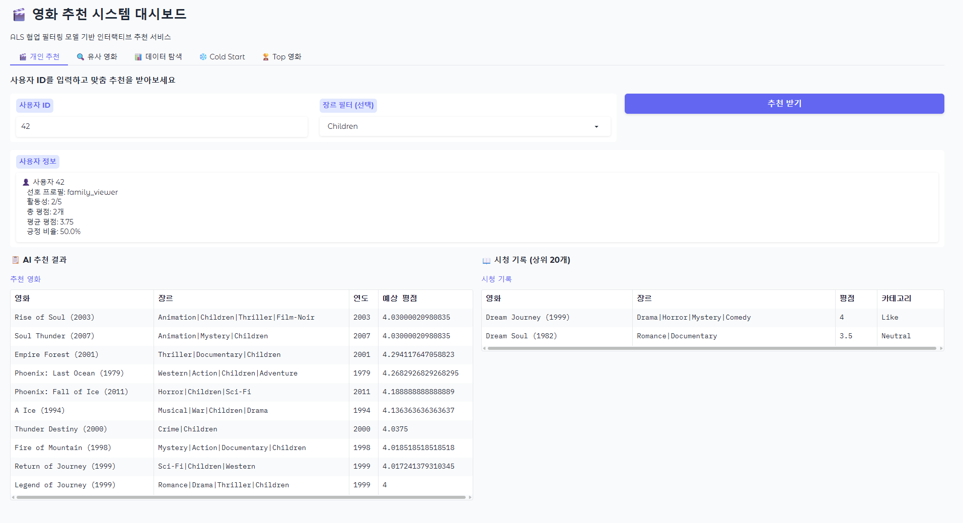

전체 흐름

01_generate_sample_data → 샘플 데이터 생성
02_silver_layer_transformation → 정제 + feature 생성
03_gold_layer_and_als_model → 집계 + ALS 학습 + MLflow 등록
04_recommendation_service → 추천 서비스 로직 + 분석 + 통계 표 output
05_recommendation_dashboard → 시각화 + Gradio 대시보드

NYC_Taxi_201912 실습

Exploring sample NYC Taxi Data from Databricks

Based on Databricks Sample Presentation
Albert Nogués 2021.

We will load some sample data from the NYC taxi dataset available in databricks, load them and store them as table. We will use then python to do some manipulation (Extract month and year from the trip time), which will create two new additional columns to our dataframe and will check how the file is saved in the hive warehouse. We will observe we have some junk data as it created folders for months and years (partitioning), that we are not supposed to have, so we will use filter to apply some filter in python way and in sql way to filter these bad records

Then, we will load another month of data as a temporary view and will compare this in contrast with a delta table where we can run updates and all sort of DML.

As a last step, we will load some master data and will perform a join. For more on Delta Lake you can follow this tutorial --> https://delta.io/tutorials/delta-lake-workshop-primer/

%fs
ls dbfs:/databricks-datasets/nyctaxi/tripdata/yellow

output

path	name	size	modificationTime
dbfs:/databricks-datasets/nyctaxi/tripdata/yellow/yellow_tripdata_2009-01.csv.gz	yellow_tripdata_2009-01.csv.gz	504262564	1590525201000
dbfs:/databricks-datasets/nyctaxi/tripdata/yellow/yellow_tripdata_2009-02.csv.gz	yellow_tripdata_2009-02.csv.gz	480034681	1590525201000
dbfs:/databricks-datasets/nyctaxi/tripdata/yellow/yellow_tripdata_2009-03.csv.gz	yellow_tripdata_2009-03.csv.gz	521102719	1590525201000
dbfs:/databricks-datasets/nyctaxi/tripdata/yellow/yellow_tripdata_2009-04.csv.gz	yellow_tripdata_2009-04.csv.gz	515435466	1590525201000
dbfs:/databricks-datasets/nyctaxi/tripdata/yellow/yellow_tripdata_2009-05.csv.gz	yellow_tripdata_2009-05.csv.gz	531133739	1590525201000

... (이하 생략)

# 파일 메타데이터를 데이터프레임으로 불러오기
df = spark.read.format("binaryFile").load("dbfs:/databricks-datasets/nyctaxi/tripdata/yellow/")

# 임시 뷰로 등록
df.createOrReplaceTempView("file_metadata")

%sql
SELECT 
    SUM(length) AS total_size_bytes,
    SUM(length) / 1024 AS total_size_kb,
    SUM(length) / (1024 * 1024) AS total_size_mb,
    SUM(length) / (1024 * 1024 * 1024) AS total_size_gb
FROM file_metadata

output

total_size_bytes	total_size_kb	total_size_mb	total_size_gb
50244255636	49066655.89453125	47916.656147003174	46.79360951855779

We define the scructure of the dataframe (columns: names and types), and create a new dataframe with this schema for us to analyze through spark

StructType 및 StructField: 각 데이터 컬럼의 타입을 지정합니다.
컬럼 이름 및 타입: NYC 택시 데이터의 각 필드를 정의하며, Vendor는 택시 회사, Pickup_DateTime은 탑승 시간, Dropoff_DateTime은 하차 시간 등으로 구성됩니다. 각 필드는 StringType, IntegerType, DoubleType, TimestampType 등으로 지정되어 있습니다.
True 값: 각 필드가 nullable(빈 값 허용)이 가능한지를 나타냅니다.

rawDF 데이터프레임에는 2019년 12월 NYC 택시 데이터가 담기며, 이후 다양한 분석 작업에 활용할 수 있습니다.

from pyspark.sql.functions import col, lit, expr, when
from pyspark.sql.types import *
from datetime import datetime
import time

# Define schema
nyc_schema = StructType([
  StructField('Vendor', StringType(), True),
  StructField('Pickup_DateTime', TimestampType(), True),
  StructField('Dropoff_DateTime', TimestampType(), True),
  StructField('Passenger_Count', IntegerType(), True),
  StructField('Trip_Distance', DoubleType(), True),
  StructField('Pickup_Longitude', DoubleType(), True),
  StructField('Pickup_Latitude', DoubleType(), True),
  StructField('Rate_Code', StringType(), True),
  StructField('Store_And_Forward', StringType(), True),
  StructField('Dropoff_Longitude', DoubleType(), True),
  StructField('Dropoff_Latitude', DoubleType(), True),
  StructField('Payment_Type', StringType(), True),
  StructField('Fare_Amount', DoubleType(), True),
  StructField('Surcharge', DoubleType(), True),
  StructField('MTA_Tax', DoubleType(), True),
  StructField('Tip_Amount', DoubleType(), True),
  StructField('Tolls_Amount', DoubleType(), True),
  StructField('Total_Amount', DoubleType(), True)
])

rawDF = spark.read.format('csv').options(header=True).schema(nyc_schema).load("dbfs:/databricks-datasets/nyctaxi/tripdata/yellow/yellow_tripdata_2019-12.csv.gz")

rawDF.take(5)

#take(5) 함수는 rawDF 데이터프레임에서 상위 5개의 행을 가져옵니다. 이 함수는 데이터를 작은 목록으로 반환하므로, 데이터의 구조를 빠르게 확인하거나 일부 데이터 샘플을 살펴볼 때 유용합니다.

#The take(5) function retrieves the top 5 rows from the rawDF DataFrame. This function returns the data as a small list, making it helpful for quickly checking the data structure or examining a small sample of the data.

output

[Row(Vendor='1', Pickup_DateTime=datetime.datetime(2019, 12, 1, 0, 26, 58), Dropoff_DateTime=datetime.datetime(2019, 12, 1, 0, 41, 45), Passenger_Count=1, Trip_Distance=4.2, Pickup_Longitude=1.0, Pickup_Latitude=None, Rate_Code='142', Store_And_Forward='116', Dropoff_Longitude=2.0, Dropoff_Latitude=14.5, Payment_Type='3', Fare_Amount=0.5, Surcharge=0.0, MTA_Tax=0.0, Tip_Amount=0.3, Tolls_Amount=18.3, Total_Amount=2.5),
 Row(Vendor='1', Pickup_DateTime=datetime.datetime(2019, 12, 1, 0, 12, 8), Dropoff_DateTime=datetime.datetime(2019, 12, 1, 0, 12, 14), Passenger_Count=1, Trip_Distance=0.0, Pickup_Longitude=1.0, Pickup_Latitude=None, Rate_Code='145', Store_And_Forward='145', Dropoff_Longitude=2.0, Dropoff_Latitude=2.5, Payment_Type='0.5', Fare_Amount=0.5, Surcharge=0.0, MTA_Tax=0.0, Tip_Amount=0.3, Tolls_Amount=3.8, Total_Amount=0.0),
 Row(Vendor='1', Pickup_DateTime=datetime.datetime(2019, 12, 1, 0, 25, 53), Dropoff_DateTime=datetime.datetime(2019, 12, 1, 0, 26, 4), Passenger_Count=1, Trip_Distance=0.0, Pickup_Longitude=1.0, Pickup_Latitude=None, Rate_Code='145', Store_And_Forward='145', Dropoff_Longitude=2.0, Dropoff_Latitude=2.5, Payment_Type='0.5', Fare_Amount=0.5, Surcharge=0.0, MTA_Tax=0.0, Tip_Amount=0.3, Tolls_Amount=3.8, Total_Amount=0.0),
 Row(Vendor='1', Pickup_DateTime=datetime.datetime(2019, 12, 1, 0, 12, 3), Dropoff_DateTime=datetime.datetime(2019, 12, 1, 0, 33, 19), Passenger_Count=2, Trip_Distance=9.4, Pickup_Longitude=1.0, Pickup_Latitude=None, Rate_Code='138', Store_And_Forward='25', Dropoff_Longitude=1.0, Dropoff_Latitude=28.5, Payment_Type='0.5', Fare_Amount=0.5, Surcharge=10.0, MTA_Tax=0.0, Tip_Amount=0.3, Tolls_Amount=39.8, Total_Amount=0.0),
 Row(Vendor='1', Pickup_DateTime=datetime.datetime(2019, 12, 1, 0, 5, 27), Dropoff_DateTime=datetime.datetime(2019, 12, 1, 0, 16, 32), Passenger_Count=2, Trip_Distance=1.6, Pickup_Longitude=1.0, Pickup_Latitude=None, Rate_Code='161', Store_And_Forward='237', Dropoff_Longitude=2.0, Dropoff_Latitude=9.0, Payment_Type='3', Fare_Amount=0.5, Surcharge=0.0, MTA_Tax=0.0, Tip_Amount=0.3, Tolls_Amount=12.8, Total_Amount=2.5)]

rawDF.printSchema()

#printSchema() 함수는 rawDF 데이터프레임의 스키마(데이터 구조)를 출력합니다. 각 컬럼의 이름, 데이터 타입, null 값 허용 여부 등을 확인할 수 있습니다. 이는 데이터셋의 구조를 이해하고, 특정 컬럼에 대한 타입이나 속성을 미리 파악하는 데 유용합니다.

#The printSchema() function prints the schema (data structure) of the rawDF DataFrame. It displays each column's name, data type, and whether null values are allowed. This is useful for understanding the dataset structure and quickly identifying the types and properties of specific columns.

output

root
 |-- Vendor: string (nullable = true)
 |-- Pickup_DateTime: timestamp (nullable = true)
 |-- Dropoff_DateTime: timestamp (nullable = true)
 |-- Passenger_Count: integer (nullable = true)
 |-- Trip_Distance: double (nullable = true)
 |-- Pickup_Longitude: double (nullable = true)
 |-- Pickup_Latitude: double (nullable = true)
 |-- Rate_Code: string (nullable = true)
 |-- Store_And_Forward: string (nullable = true)
 |-- Dropoff_Longitude: double (nullable = true)
 |-- Dropoff_Latitude: double (nullable = true)
 |-- Payment_Type: string (nullable = true)
 |-- Fare_Amount: double (nullable = true)
 |-- Surcharge: double (nullable = true)
 |-- MTA_Tax: double (nullable = true)
 |-- Tip_Amount: double (nullable = true)
 |-- Tolls_Amount: double (nullable = true)
 |-- Total_Amount: double (nullable = true)

CREATE taxidata DATABASE and taxi_2019_12 Table

CREATE DATABASE IF NOT EXISTS taxidata : taxidata라는 데이터베이스가 존재하지 않을 경우, 이를 새로 생성합니다. 이렇게 하면 NYC 택시 데이터를 위한 별도의 데이터베이스를 만들 수 있습니다.

DROP TABLE IF EXISTS taxidata.taxi_2019_12: taxidata 데이터베이스 내에 taxi_2019_12라는 테이블이 이미 존재한다면 이를 삭제합니다. 이 과정은 데이터를 처음부터 새로 삽입할 수 있도록 기존 테이블을 제거하는 초기화 작업입니다.

CREATE DATABASE IF NOT EXISTS taxidata; creates a new database called taxidata if it does not already exist. This is useful for organizing NYC taxi data in a dedicated database.

DROP TABLE IF EXISTS taxidata.taxi_2019_12; deletes the taxi_2019_12 table within the taxidata database if it already exists. This step resets the table, allowing data to be reloaded from scratch.

%sql
CREATE DATABASE IF NOT EXISTS taxidata;
DROP TABLE IF EXISTS taxidata.taxi_2019_12;

output

| |
||

%python
#rawDF 데이터프레임의 데이터를 taxidata 데이터베이스 내의 taxi_2019_12 테이블에 저장합니다.
#This code saves the data from the rawDF DataFrame to the taxi_2019_12 table within the taxidata database.

rawDF.write.mode("overwrite").saveAsTable("taxidata.taxi_2019_12")

# .write는 데이터프레임을 저장할 때 사용하는 메서드입니다.
# mode("overwrite")는 기존 테이블이 있을 경우 덮어쓰도록 지정합니다. 즉, 동일한 이름의 테이블이 이미 존재하면 그 테이블을 삭제하고 새 데이터를 덮어씁니다. 이는 데이터 업데이트가 필요한 경우 유용합니다.
# saveAsTable("taxidata.taxi_2019_12")는 taxidata 데이터베이스의 taxi_2019_12 테이블에 데이터를 저장하는 명령입니다.

# .write is used to initiate the save process for the DataFrame data.
# mode("overwrite") specifies that if the table already exists, it should be overwritten. This effectively deletes any existing table with the same name and replaces it with the new data, making it useful for data updates.
# saveAsTable("taxidata.taxi_2019_12") saves the data into the taxi_2019_12 table within the taxidata database.

%sql
-- can use sql because table is created.

describe taxidata.taxi_2019_12

output

col_name	data_type	comment
Vendor	string
Pickup_DateTime	timestamp
Dropoff_DateTime	timestamp
Passenger_Count	int
Trip_Distance	double

... (이하 생략)

%fs
rm -r /delta/taxi

output

<div class="ansiout">res1: Boolean = false
</div>

Saves the NYC taxi data in Delta format

이 코드는 NYC 택시 데이터를 Delta 형식으로 저장하고, 연도와 월 기준으로 파티셔닝하여 저장 위치에 관리할 수 있게 합니다.

withColumn('Year', expr('cast(year(Pickup_DateTime) as int)')): Pickup_DateTime 컬럼에서 연도를 추출하여 Year라는 새 컬럼을 추가합니다.
withColumn('Month', expr('cast(month(Pickup_DateTime) as int)')): Pickup_DateTime 컬럼에서 월을 추출하여 Month라는 새 컬럼을 추가합니다.
processedDF.write.format('delta'): 데이터프레임을 Delta 형식으로 저장합니다.
mode('append'): 기존 데이터에 추가하여 저장합니다. 이미 같은 경로에 데이터가 있더라도 덮어쓰지 않고 새로운 데이터를 추가합니다.
partitionBy('Year','Month'): 데이터를 Year와 Month 컬럼으로 파티셔닝하여 저장합니다. 이렇게 하면 연도와 월별로 데이터가 분할되어 저장되므로, 특정 연도나 월에 대해 데이터를 효율적으로 조회할 수 있습니다.
save("/delta/taxi"): Delta 테이블의 저장 경로로 /delta/taxi를 지정합니다.

#####English Explanation
This code saves the NYC taxi data in Delta format, partitioned by year and month, making it more manageable and query-efficient.

withColumn('Year', expr('cast(year(Pickup_DateTime) as int)')): Adds a new column Year by extracting the year from the Pickup_DateTime column.
withColumn('Month', expr('cast(month(Pickup_DateTime) as int)')): Adds a new column Month by extracting the month from the Pickup_DateTime column.
processedDF.write.format('delta'): Specifies Delta format for saving the DataFrame.
mode('append'): Appends data to the existing dataset, adding new data without overwriting.
partitionBy('Year','Month'): Partitions the data by Year and Month columns, making it more efficient for queries targeting specific years or months.
save("/delta/taxi"): Sets /delta/taxi as the storage location for the Delta table.

processedDF = rawDF.withColumn('Year', expr('cast(year(Pickup_DateTime) as int)')).withColumn('Month', expr('cast(month(Pickup_DateTime) as int)')) 
processedDF.write.format('delta').mode('append').partitionBy('Year','Month').save("/delta/taxi")

display(processedDF)

output

Vendor	Pickup_DateTime	Dropoff_DateTime	Passenger_Count	Trip_Distance	Pickup_Longitude	Rate_Code	Store_And_Forward	Dropoff_Longitude	Dropoff_Latitude	Payment_Type	Fare_Amount	Surcharge	Tip_Amount	Tolls_Amount	Total_Amount	Year	Month
1	2019-12-01T00:26:58Z	2019-12-01T00:41:45Z	1	4.2	1.0	142	116	2.0	14.5	3	0.5	0.0	0.3	18.3	2.5	2019	12
1	2019-12-01T00:12:08Z	2019-12-01T00:12:14Z	1	0.0	1.0	145	145	2.0	2.5	0.5	0.5	0.0	0.3	3.8	0.0	2019	12
1	2019-12-01T00:25:53Z	2019-12-01T00:26:04Z	1	0.0	1.0	145	145	2.0	2.5	0.5	0.5	0.0	0.3	3.8	0.0	2019	12
1	2019-12-01T00:12:03Z	2019-12-01T00:33:19Z	2	9.4	1.0	138	25	1.0	28.5	0.5	0.5	10.0	0.3	39.8	0.0	2019	12
1	2019-12-01T00:05:27Z	2019-12-01T00:16:32Z	2	1.6	1.0	161	237	2.0	9.0	3	0.5	0.0	0.3	12.8	2.5	2019	12

... (이하 생략)

%fs
ls dbfs:/delta/taxi

output

path	name	modificationTime
dbfs:/delta/taxi/Year=2008/	Year=2008/	1774581345000
dbfs:/delta/taxi/Year=2009/	Year=2009/	1774581345000
dbfs:/delta/taxi/Year=2019/	Year=2019/	1774581340000
dbfs:/delta/taxi/Year=2020/	Year=2020/	1774581340000
dbfs:/delta/taxi/Year=2026/	Year=2026/	1774581344000

... (이하 생략)

위의 결과를 보면, dbfs:/delta/taxi 경로에 연도별 파티션 폴더들이 생성되어 있습니다.

Year=2008, Year=2009 등 예상치 못한 연도 폴더들이 보이는 이유는 다음과 같은 원인이 있을 수 있습니다:

(1) 잘못된 데이터 입력: Pickup_DateTime 컬럼에 잘못된 연도가 포함된 데이터가 있을 수 있습니다. 예를 들어, 데이터가 잘못 입력되어 2008년이나 2090년 같은 값이 들어갔을 수 있습니다.

(2) 데이터 전처리 과정의 오류: 데이터 생성 또는 로딩 중에 Pickup_DateTime 값이 잘못 파싱되었을 수 있습니다. 이로 인해 실제 존재하지 않는 미래 연도나 과거 연도로 분류되었을 가능성이 있습니다.

(3) 테스트 데이터 포함:데이터에 테스트 또는 샘플 데이터가 포함되어 있을 수 있으며, 이 데이터들이 실제 연도 범위를 벗어나는 값을 가질 수 있습니다.

이 문제를 해결하려면, 데이터에서 예상하지 못한 연도 값을 가진 레코드를 필터링하거나 Pickup_DateTime 컬럼의 값이 적절한지 확인하는 추가적인 검증 작업을 수행해야 합니다.

====================

English Explanation

Year-partitioned folders have been created in the dbfs:/delta/taxi path. Here are possible reasons why unexpected year folders like Year=2008, Year=2009 appear:

(1) Incorrect Data Entry: There may be data with incorrect years in the Pickup_DateTime column. For example, data might have been incorrectly entered with years like 2008 or 2090.

(2) Data Preprocessing Errors: The Pickup_DateTime values might have been parsed incorrectly during data generation or loading. This could have resulted in classification into non-existent future years or past years.

(3) Inclusion of Test Data: The dataset may include test or sample data, and these records might contain values outside the expected year range.

To resolve this issue, you need to either filter out records with unexpected year values or perform additional validation checks to ensure the values in the Pickup_DateTime column are appropriate.

%fs
ls dbfs:/delta/taxi/Year=2019/Month=12/

output

path	name	size	modificationTime
dbfs:/delta/taxi/Year=2019/Month=12/part-00000-808ad32a-4c70-4f98-98ac-b7c5bed198f4.c000.snappy.parquet	part-00000-808ad32a-4c70-4f98-98ac-b7c5bed198f4.c000.snappy.parquet	145070651	1774581343000

%fs
ls dbfs:/delta/taxi/Year=2019/Month=11/

output

path	name	size	modificationTime
dbfs:/delta/taxi/Year=2019/Month=11/part-00000-a7db0d34-c292-42fb-b373-bd2af6a2ba90.c000.snappy.parquet	part-00000-a7db0d34-c292-42fb-b373-bd2af6a2ba90.c000.snappy.parquet	10560	1774581344000

#So we found some dirty data in our dataframe! we can filter it.
processedDF.filter("year=2019").count() #the SQL way!

output

#from pyspark.sql import functions as F
from pyspark.sql.functions import col, lit, expr, when
from pyspark.sql.types import *

processedDF.filter((col('Year')==2019) & (col('Month')==12)).count() # Dataframe way!

output

processedDF.createOrReplaceTempView("taxi_data_view")
spark.sql("SELECT COUNT(*) FROM taxi_data_view WHERE Year = 2019 AND Month = 12").show()

output

+--------+
|count(1)|
+--------+
| 6895933|
+--------+

%sql
SELECT COUNT(*) FROM taxi_data_view WHERE Year = 2019 AND Month = 12

output

count(1)
6895933

processedDF.filter((col('Year')!=2019) & (col('Month')!=12)).count()

output

processedDF.filter("Year <> 2019 and Month <> 12").count() #The SQL Way

output

%sql
use taxidata;
show tables;

output

database	tableName	isTemporary
taxidata	taxi_2019_12	False
	_sqldf	True
	file_metadata	True
	taxi_data_view	True

Save Cleaned Data in Delta format

다음 코드는 processedDF 데이터프레임에서 Year가 2019이고 Month가 12인 데이터만 필터링하여 Delta 형식으로 /delta/taxiclean 경로에 저장합니다.

filter("Year = 2019 and Month = 12"): Selects rows where Year is 2019 and Month is 12.
.write.format('delta'): Specifies that the data should be saved in Delta format.
mode('overwrite'): Sets the mode to overwrite, so any existing data in /delta/taxiclean will be replaced.
partitionBy('Year','Month'): Partitions the data by Year and Month, making queries targeting specific years and months more efficient.
save("/delta/taxiclean"): Specifies /delta/taxiclean as the storage path for the Delta table.

%fs
rm -r /delta/taxiclean

output

<div class="ansiout">res5: Boolean = false
</div>

%python
processedDF.filter("Year = 2019 and Month = 12").write.format('delta').mode('overwrite').partitionBy('Year','Month').save("/delta/taxiclean")

processedDF.filter("Year <> 2019 and Month <> 12") \
    .write.mode('overwrite') \
    .saveAsTable("taxidata.taxi_excluding_dec_2019")

%fs
ls dbfs:/delta/taxiclean/

output

path	name	size	modificationTime
dbfs:/delta/taxiclean/Year=2019/	Year=2019/	0	1774581422000
dbfs:/delta/taxiclean/_delta_log/	_delta_log/	0	1774581422000

# Read Delta Table : Delta 테이블을 DataFrame으로 로드
taxi_clean_df = spark.read.format("delta").load("/delta/taxiclean")

# 데이터 샘플 확인
taxi_clean_df.show(5)

output

+------+-------------------+-------------------+---------------+-------------+----------------+---------------+---------+-----------------+-----------------+----------------+------------+-----------+---------+-------+----------+------------+------------+----+-----+
|Vendor|    Pickup_DateTime|   Dropoff_DateTime|Passenger_Count|Trip_Distance|Pickup_Longitude|Pickup_Latitude|Rate_Code|Store_And_Forward|Dropoff_Longitude|Dropoff_Latitude|Payment_Type|Fare_Amount|Surcharge|MTA_Tax|Tip_Amount|Tolls_Amount|Total_Amount|Year|Month|
+------+-------------------+-------------------+---------------+-------------+----------------+---------------+---------+-----------------+-----------------+----------------+------------+-----------+---------+-------+----------+------------+------------+----+-----+
|     1|2019-12-01 00:26:58|2019-12-01 00:41:45|              1|          4.2|             1.0|           NULL|      142|              116|              2.0|            14.5|           3|        0.5|      0.0|    0.0|       0.3|        18.3|         2.5|2019|   12|
|     1|2019-12-01 00:12:08|2019-12-01 00:12:14|              1|          0.0|             1.0|           NULL|      145|              145|              2.0|             2.5|         0.5|        0.5|      0.0|    0.0|       0.3|         3.8|         0.0|2019|   12|
|     1|2019-12-01 00:25:53|2019-12-01 00:26:04|              1|          0.0|             1.0|           NULL|      145|              145|              2.0|             2.5|         0.5|        0.5|      0.0|    0.0|       0.3|         3.8|         0.0|2019|   12|
|     1|2019-12-01 00:12:03|2019-12-01 00:33:19|              2|          9.4|             1.0|           NULL|      138|               25|              1.0|            28.5|         0.5|        0.5|     10.0|    0.0|       0.3|        39.8|         0.0|2019|   12|
|     1|2019-12-01 00:05:27|2019-12-01 00:16:32|              2|          1.6|             1.0|           NULL|      161|              237|              2.0|             9.0|           3|        0.5|      0.0|    0.0|       0.3|        12.8|         2.5|2019|   12|
+------+-------------------+-------------------+---------------+-------------+----------------+---------------+---------+-----------------+-----------------+----------------+------------+-----------+---------+-------+----------+------------+------------+----+-----+
only showing top 5 rows

# or in the SQL way, you can read delta table
spark.sql("SELECT * FROM delta.`/delta/taxiclean`")
display(spark.sql("SELECT * FROM delta.`/delta/taxiclean`"))

output

Vendor	Pickup_DateTime	Dropoff_DateTime	Passenger_Count	Trip_Distance	Pickup_Longitude	Rate_Code	Store_And_Forward	Dropoff_Longitude	Dropoff_Latitude	Payment_Type	Fare_Amount	Surcharge	Tip_Amount	Tolls_Amount	Total_Amount	Year	Month
1	2019-12-01T00:26:58Z	2019-12-01T00:41:45Z	1	4.2	1.0	142	116	2.0	14.5	3	0.5	0.0	0.3	18.3	2.5	2019	12
1	2019-12-01T00:12:08Z	2019-12-01T00:12:14Z	1	0.0	1.0	145	145	2.0	2.5	0.5	0.5	0.0	0.3	3.8	0.0	2019	12
1	2019-12-01T00:25:53Z	2019-12-01T00:26:04Z	1	0.0	1.0	145	145	2.0	2.5	0.5	0.5	0.0	0.3	3.8	0.0	2019	12
1	2019-12-01T00:12:03Z	2019-12-01T00:33:19Z	2	9.4	1.0	138	25	1.0	28.5	0.5	0.5	10.0	0.3	39.8	0.0	2019	12
1	2019-12-01T00:05:27Z	2019-12-01T00:16:32Z	2	1.6	1.0	161	237	2.0	9.0	3	0.5	0.0	0.3	12.8	2.5	2019	12

... (이하 생략)

# 통계 정보 확인
taxi_clean_df.select("Fare_Amount", "Tip_Amount", "Total_Amount").describe().show()

output

+-------+-------------------+--------------------+------------------+
|summary|        Fare_Amount|          Tip_Amount|      Total_Amount|
+-------+-------------------+--------------------+------------------+
|  count|            6895933|             6895933|           6895933|
|   mean| 0.4924146826832601| 0.29798568231785594| 2.275278631622436|
| stddev|0.07233884348175239|0.033814608330983875|0.7359655528934228|
|    min|               -0.5|                -0.3|              -2.5|
|    max|                3.3|                 0.3|               3.0|
+-------+-------------------+--------------------+------------------+

# 특정 조건으로 필터링
long_trips_df = taxi_clean_df.filter(taxi_clean_df.Trip_Distance > 10)
long_trips_df.show(5)

output

+------+-------------------+-------------------+---------------+-------------+----------------+---------------+---------+-----------------+-----------------+----------------+------------+-----------+---------+-------+----------+------------+------------+----+-----+
|Vendor|    Pickup_DateTime|   Dropoff_DateTime|Passenger_Count|Trip_Distance|Pickup_Longitude|Pickup_Latitude|Rate_Code|Store_And_Forward|Dropoff_Longitude|Dropoff_Latitude|Payment_Type|Fare_Amount|Surcharge|MTA_Tax|Tip_Amount|Tolls_Amount|Total_Amount|Year|Month|
+------+-------------------+-------------------+---------------+-------------+----------------+---------------+---------+-----------------+-----------------+----------------+------------+-----------+---------+-------+----------+------------+------------+----+-----+
|     2|2019-12-01 00:43:02|2019-12-01 01:11:18|              1|        13.07|             1.0|           NULL|       41|               51|              2.0|            38.5|         0.5|        0.5|      0.0|    0.0|       0.3|        39.8|         0.0|2019|   12|
|     1|2019-12-01 00:04:40|2019-12-01 00:31:27|              0|         17.4|             2.0|           NULL|      132|              141|              1.0|            52.0|         2.5|        0.5|     5.53|    0.0|       0.3|       60.83|         2.5|2019|   12|
|     2|2019-12-01 00:37:17|2019-12-01 01:07:39|              5|        19.98|             2.0|           NULL|      132|              238|              1.0|            52.0|           0|        0.5|    14.73|   6.12|       0.3|       73.65|         0.0|2019|   12|
|     1|2019-12-01 00:43:27|2019-12-01 01:23:30|              1|         23.5|             4.0|           NULL|       68|              265|              1.0|            85.5|           3|        0.5|    17.85|    0.0|       0.3|      107.15|         2.5|2019|   12|
|     1|2019-12-01 00:43:09|2019-12-01 01:11:07|              2|         11.3|             1.0|           NULL|      138|               85|              1.0|            33.5|         0.5|        0.5|     6.95|    0.0|       0.3|       41.75|         0.0|2019|   12|
+------+-------------------+-------------------+---------------+-------------+----------------+---------------+---------+-----------------+-----------------+----------------+------------+-----------+---------+-------+----------+------------+------------+----+-----+
only showing top 5 rows

display(long_trips_df.limit(5))

output

Vendor	Pickup_DateTime	Dropoff_DateTime	Passenger_Count	Trip_Distance	Pickup_Longitude	Rate_Code	Store_And_Forward	Dropoff_Longitude	Dropoff_Latitude	Payment_Type	Fare_Amount	Surcharge	MTA_Tax	Tip_Amount	Tolls_Amount	Total_Amount	Year	Month
2	2019-12-01T00:43:02Z	2019-12-01T01:11:18Z	1	13.07	1.0	41	51	2.0	38.5	0.5	0.5	0.0	0.0	0.3	39.8	0.0	2019	12
1	2019-12-01T00:04:40Z	2019-12-01T00:31:27Z	0	17.4	2.0	132	141	1.0	52.0	2.5	0.5	5.53	0.0	0.3	60.83	2.5	2019	12
2	2019-12-01T00:37:17Z	2019-12-01T01:07:39Z	5	19.98	2.0	132	238	1.0	52.0	0	0.5	14.73	6.12	0.3	73.65	0.0	2019	12
1	2019-12-01T00:43:27Z	2019-12-01T01:23:30Z	1	23.5	4.0	68	265	1.0	85.5	3	0.5	17.85	0.0	0.3	107.15	2.5	2019	12
1	2019-12-01T00:43:09Z	2019-12-01T01:11:07Z	2	11.3	1.0	138	85	1.0	33.5	0.5	0.5	6.95	0.0	0.3	41.75	0.0	2019	12

###이제 NYC 택시 데이터의 2019년 11월 데이터를 읽어와 rawDF2라는 데이터프레임에 로드합니다.

spark.read.format('csv'): 데이터를 CSV 형식으로 읽도록 지정합니다.
options(header=True): 첫 번째 행을 헤더로 인식합니다.
schema(nyc_schema): 이전에 정의한 nyc_schema 스키마를 사용하여 각 컬럼의 타입을 미리 지정합니다.
load("dbfs:/databricks-datasets/nyctaxi/tripdata/yellow/yellow_tripdata_2019-11.csv.gz"): 지정된 경로에서 압축된 CSV 파일을 불러옵니다.

Lazy Execution (지연 실행): Spark에서는 데이터프레임에 대한 변환(transformation) 작업이 즉시 실행되지 않습니다. 데이터는 필요할 때(예: show(), count() 등 액션을 호출할 때)까지 로드되지 않으므로 메모리와 처리 속도를 효율적으로 사용할 수 있습니다. 여기서 rawDF2는 지연 실행 방식으로 정의되며, 실제 데이터 로드는 액션을 호출할 때 발생합니다.

English Explanation:
This code reads the November 2019 NYC taxi data into a DataFrame named rawDF2.

spark.read.format('csv'): Specifies reading data in CSV format.
options(header=True): Recognizes the first row as headers.
schema(nyc_schema): Applies the pre-defined schema nyc_schema to set data types for each column.
load("dbfs:/databricks-datasets/nyctaxi/tripdata/yellow/yellow_tripdata_2019-11.csv.gz"): Loads the compressed CSV file from the specified path.

Lazy Execution: In Spark, transformations on DataFrames are not executed immediately. Data loading and computation happen only when an action (like show() or count()) is called, which optimizes memory and processing speed. Here, rawDF2 is defined with lazy execution, meaning the data is loaded only when an action is triggered.

rawDF2 = spark.read.format('csv').options(header=True).schema(nyc_schema).load("dbfs:/databricks-datasets/nyctaxi/tripdata/yellow/yellow_tripdata_2019-11.csv.gz") #Lazy Execution

rawDF2.createOrReplaceTempView("taxi_2019_11_tmp")

%sql
--use taxidata;
show tables

output

database	tableName	isTemporary
taxidata	taxi_2019_12	False
taxidata	taxi_excluding_dec_2019	False
	_sqldf	True
	file_metadata	True
	taxi_2019_11_tmp	True

... (이하 생략)

%python
rawDF2.take(1)

output

[Row(Vendor='1', Pickup_DateTime=datetime.datetime(2019, 11, 1, 0, 30, 41), Dropoff_DateTime=datetime.datetime(2019, 11, 1, 0, 32, 25), Passenger_Count=1, Trip_Distance=0.0, Pickup_Longitude=1.0, Pickup_Latitude=None, Rate_Code='145', Store_And_Forward='145', Dropoff_Longitude=2.0, Dropoff_Latitude=3.0, Payment_Type='0.5', Fare_Amount=0.5, Surcharge=0.0, MTA_Tax=0.0, Tip_Amount=0.3, Tolls_Amount=4.3, Total_Amount=0.0)]

%sql
drop table if exists taxidata.taxi;

Create 
TABLE taxidata.taxi 
As 
Select * from taxidata.taxi_2019_12 limit 1;

output

num_affected_rows	num_inserted_rows

%sql
select count (*) from taxidata.taxi;

output

count(1)
1

%sql
select * from taxidata.taxi;

output

Vendor	Pickup_DateTime	Dropoff_DateTime	Passenger_Count	Trip_Distance	Pickup_Longitude	Pickup_Latitude	Rate_Code	Store_And_Forward	Dropoff_Longitude	Dropoff_Latitude	Payment_Type	Fare_Amount	Surcharge	MTA_Tax	Tip_Amount	Tolls_Amount	Total_Amount
1	2019-12-01T00:26:58Z	2019-12-01T00:41:45Z	1	4.2	1.0		142	116	2.0	14.5	3	0.5	0.0	0.0	0.3	18.3	2.5

%sql
UPDATE taxidata.taxi 
set vendor=0 
where vendor =1;

--taxidata.taxi is a table, so it's updatable.

output

num_affected_rows
1

%sql
select * from taxidata.taxi;

output

Vendor	Pickup_DateTime	Dropoff_DateTime	Passenger_Count	Trip_Distance	Pickup_Longitude	Pickup_Latitude	Rate_Code	Store_And_Forward	Dropoff_Longitude	Dropoff_Latitude	Payment_Type	Fare_Amount	Surcharge	MTA_Tax	Tip_Amount	Tolls_Amount	Total_Amount
0	2019-12-01T00:26:58Z	2019-12-01T00:41:45Z	1	4.2	1.0		142	116	2.0	14.5	3	0.5	0.0	0.0	0.3	18.3	2.5

%sql
UPDATE taxi_2019_11_tmp 
set vendor=0 
where vendor =1; 
-- Not working. Only DELTA tables can be updated. Need to create derivate dataframes or other temp tables and persist them as delta
--taxi_2019_11_tmp is a temp view

%fs
ls dbfs:/databricks-datasets/nyctaxi/taxizone/

output

path	name	size	modificationTime
dbfs:/databricks-datasets/nyctaxi/taxizone/taxi_payment_type.csv	taxi_payment_type.csv	93	1590524947000
dbfs:/databricks-datasets/nyctaxi/taxizone/taxi_rate_code.csv	taxi_rate_code.csv	109	1590524947000
dbfs:/databricks-datasets/nyctaxi/taxizone/taxi_zone_lookup.csv	taxi_zone_lookup.csv	12322	1590524947000

dbutils.fs.head("dbfs:/databricks-datasets/nyctaxi/taxizone/taxi_payment_type.csv")

output

'payment_type,payment_desc\n1,Credit card\n2,Cash\n3,No Charge\n4,Dispute\n5,Unknown\n6,Voided trip\n'

paymentTypeDF = spark.read.format('csv') \
  .options(header=True) \
  .options(inferSchema=True) \
  .load("dbfs:/databricks-datasets/nyctaxi/taxizone/taxi_payment_type.csv") 
  #small file, we can use inferSchema to see if Spark is capable to get the right datatypes so we avoid having to define a schema for this dataframe

display(paymentTypeDF)

output

payment_type	payment_desc
1	Credit card
2	Cash
3	No Charge
4	Dispute
5	Unknown

... (이하 생략)

#Now we want to join two tables. If we want to go with sql (first) we need to register the new dataframe as temporary table and perform the join. The second way, we will do the python way.
paymentTypeDF.createOrReplaceTempView("taxi_payment_types")

%sql

select * from taxi_payment_types;

output

payment_type	payment_desc
1	Credit card
2	Cash
3	No Charge
4	Dispute
5	Unknown

... (이하 생략)

%sql
-- We perform a join
select t.trip_distance, t.payment_type, p.payment_desc 
from taxidata.taxi t, taxi_payment_types p
where t.Payment_type = p.payment_type

output

trip_distance	payment_type	payment_desc
4.2	3	No Charge

#The Python way. I will use alias because when joining two or more dataframes with the same column name it can get messy to refer the proper column
taxiDataDF = spark.sql("select * from taxidata.taxi")
taxiDataDF.alias("t").join(paymentTypeDF.alias("p"), on=taxiDataDF.Payment_Type == paymentTypeDF.payment_type, how="inner").select("t.Trip_Distance", "t.Payment_Type", "p.Payment_Desc").show()

output

+-------------+------------+------------+
|Trip_Distance|Payment_Type|Payment_Desc|
+-------------+------------+------------+
|          4.2|           3|   No Charge|
+-------------+------------+------------+

#The Python way. I will use alias because when joining two or more dataframes with the same column name it can get messy to refer the proper column
long_trips_df.alias("t").join(paymentTypeDF.alias("p"), on=long_trips_df.Payment_Type == paymentTypeDF.payment_type, how="inner").select("t.Trip_Distance", "t.Payment_Type", "p.Payment_Desc").show()

output

+-------------+------------+------------+
|Trip_Distance|Payment_Type|Payment_Desc|
+-------------+------------+------------+
|         17.4|         2.5|        Cash|
|         23.5|           3|   No Charge|
|         12.5|           3|   No Charge|
|         19.7|         2.5|        Cash|
|         18.3|         2.5|        Cash|
|         21.0|         2.5|        Cash|
|         17.7|         2.5|        Cash|
|         17.9|         2.5|        Cash|
|         18.7|         2.5|        Cash|
|         13.7|           3|   No Charge|
|         12.1|           3|   No Charge|
|         18.0|         2.5|        Cash|
|         17.6|         2.5|        Cash|
|         20.1|         2.5|        Cash|
|         12.5|           3|   No Charge|
|         17.4|         2.5|        Cash|
|         20.9|         2.5|        Cash|
|         10.8|           3|   No Charge|
|         11.2|           3|   No Charge|
|         17.0|         2.5|        Cash|
+-------------+------------+------------+
only showing top 20 rows

display(long_trips_df.filter(long_trips_df.Payment_Type == 0.5))

output

Vendor	Pickup_DateTime	Dropoff_DateTime	Passenger_Count	Trip_Distance	Pickup_Longitude	Rate_Code	Store_And_Forward	Dropoff_Longitude	Dropoff_Latitude	Payment_Type	Fare_Amount	Surcharge	Tip_Amount	Tolls_Amount	Total_Amount	Year	Month
2	2019-12-01T00:43:02Z	2019-12-01T01:11:18Z	1	13.07	1.0	41	51	2.0	38.5	0.5	0.5	0.0	0.3	39.8	0.0	2019	12
1	2019-12-01T00:43:09Z	2019-12-01T01:11:07Z	2	11.3	1.0	138	85	1.0	33.5	0.5	0.5	6.95	0.3	41.75	0.0	2019	12
1	2019-12-01T00:48:16Z	2019-12-01T01:24:19Z	2	10.8	1.0	132	56	2.0	37.0	0.5	0.5	0.0	0.3	38.3	0.0	2019	12
2	2019-12-01T00:26:42Z	2019-12-01T01:01:01Z	5	16.53	1.0	138	14	2.0	47.0	0.5	0.5	0.0	0.3	48.3	0.0	2019	12
2	2019-12-01T00:11:21Z	2019-12-01T00:46:36Z	1	11.56	1.0	163	135	1.0	37.5	0.5	0.5	0.0	0.3	41.3	2.5	2019	12

... (이하 생략)

long_trips_df_cleaned = long_trips_df.filter(long_trips_df.Payment_Type != 0.5)
display(long_trips_df_cleaned)

output

Vendor	Pickup_DateTime	Dropoff_DateTime	Passenger_Count	Trip_Distance	Pickup_Longitude	Rate_Code	Store_And_Forward	Dropoff_Longitude	Dropoff_Latitude	Payment_Type	Fare_Amount	Surcharge	MTA_Tax	Tip_Amount	Tolls_Amount	Total_Amount	Year	Month
1	2019-12-01T00:04:40Z	2019-12-01T00:31:27Z	0	17.4	2.0	132	141	1.0	52.0	2.5	0.5	5.53	0.0	0.3	60.83	2.5	2019	12
2	2019-12-01T00:37:17Z	2019-12-01T01:07:39Z	5	19.98	2.0	132	238	1.0	52.0	0	0.5	14.73	6.12	0.3	73.65	0.0	2019	12
1	2019-12-01T00:43:27Z	2019-12-01T01:23:30Z	1	23.5	4.0	68	265	1.0	85.5	3	0.5	17.85	0.0	0.3	107.15	2.5	2019	12
1	2019-12-01T00:07:36Z	2019-12-01T00:45:26Z	1	12.5	1.0	233	14	1.0	38.5	3	0.5	8.45	0.0	0.3	50.75	2.5	2019	12
1	2019-12-01T00:12:08Z	2019-12-01T00:42:31Z	1	19.7	2.0	132	144	1.0	52.0	2.5	0.5	0.08	0.0	0.3	55.38	2.5	2019	12

... (이하 생략)

display(long_trips_df.select("Payment_Type").distinct())

output

Payment_Type
7
-1
0.3
3
4.5

... (이하 생략)

from pyspark.sql import functions as F

long_trips_df_cleaned = (
    long_trips_df
        # 1) 문자열이 정수 형태인지 정규식으로 검사: ^[0-9]+$
        .filter(F.col("Payment_Type").rlike("^[0-9]+$"))
        # 2) 정수로 캐스팅
        .withColumn("Payment_Type", F.col("Payment_Type").cast("int"))
)

display(long_trips_df_cleaned)

output

Vendor	Pickup_DateTime	Dropoff_DateTime	Passenger_Count	Trip_Distance	Pickup_Longitude	Rate_Code	Store_And_Forward	Dropoff_Longitude	Dropoff_Latitude	Payment_Type	Fare_Amount	Surcharge	MTA_Tax	Tip_Amount	Tolls_Amount	Total_Amount	Year	Month
2	2019-12-01T00:37:17Z	2019-12-01T01:07:39Z	5	19.98	2.0	132	238	1.0	52.0	0	0.5	14.73	6.12	0.3	73.65	0.0	2019	12
1	2019-12-01T00:43:27Z	2019-12-01T01:23:30Z	1	23.5	4.0	68	265	1.0	85.5	3	0.5	17.85	0.0	0.3	107.15	2.5	2019	12
1	2019-12-01T00:07:36Z	2019-12-01T00:45:26Z	1	12.5	1.0	233	14	1.0	38.5	3	0.5	8.45	0.0	0.3	50.75	2.5	2019	12
2	2019-12-01T00:20:20Z	2019-12-01T00:45:26Z	1	17.72	2.0	132	107	1.0	52.0	0	0.5	12.28	6.12	0.3	73.7	2.5	2019	12
2	2019-12-01T00:37:03Z	2019-12-01T01:11:38Z	1	20.6	2.0	132	231	2.0	52.0	0	0.5	0.0	0.0	0.3	55.3	2.5	2019	12

... (이하 생략)

display(long_trips_df_cleaned.select("Payment_Type").distinct())

output

Payment_Type
1
3
5
7
2

... (이하 생략)

from pyspark.sql import functions as F

long_trips_df_cleaned = (
    long_trips_df
        # 1) 문자열이 '정수 형태'인지 검사 → 정수 형태만 통과
        .filter(F.col("Payment_Type").rlike("^[0-9]+$"))
        # 2) 정수로 캐스팅
        .withColumn("Payment_Type", F.col("Payment_Type").try_cast("int"))
        # 3) 1~6 범위만 유지
        .filter((F.col("Payment_Type") >= 1) & (F.col("Payment_Type") <= 6))
)

display(long_trips_df_cleaned)

output

Vendor	Pickup_DateTime	Dropoff_DateTime	Passenger_Count	Trip_Distance	Pickup_Longitude	Rate_Code	Store_And_Forward	Dropoff_Longitude	Dropoff_Latitude	Payment_Type	Fare_Amount	Surcharge	MTA_Tax	Tip_Amount	Tolls_Amount	Total_Amount	Year	Month
1	2019-12-01T00:43:27Z	2019-12-01T01:23:30Z	1	23.5	4.0	68	265	1.0	85.5	3	0.5	17.85	0.0	0.3	107.15	2.5	2019	12
1	2019-12-01T00:07:36Z	2019-12-01T00:45:26Z	1	12.5	1.0	233	14	1.0	38.5	3	0.5	8.45	0.0	0.3	50.75	2.5	2019	12
1	2019-12-01T00:40:03Z	2019-12-01T01:19:53Z	1	13.7	1.0	170	11	2.0	41.5	3	0.5	0.0	0.0	0.3	45.3	2.5	2019	12
1	2019-12-01T00:54:07Z	2019-12-01T01:18:01Z	2	12.1	1.0	45	7	1.0	34.5	3	0.5	7.65	0.0	0.3	45.95	2.5	2019	12
1	2019-12-01T00:14:44Z	2019-12-01T00:38:04Z	1	12.5	1.0	162	130	2.0	35.0	3	0.5	0.0	6.12	0.3	44.92	2.5	2019	12

... (이하 생략)

display(long_trips_df_cleaned.select("Payment_Type").distinct())

output

Payment_Type
1
3
5
2

Databricks 대시보드

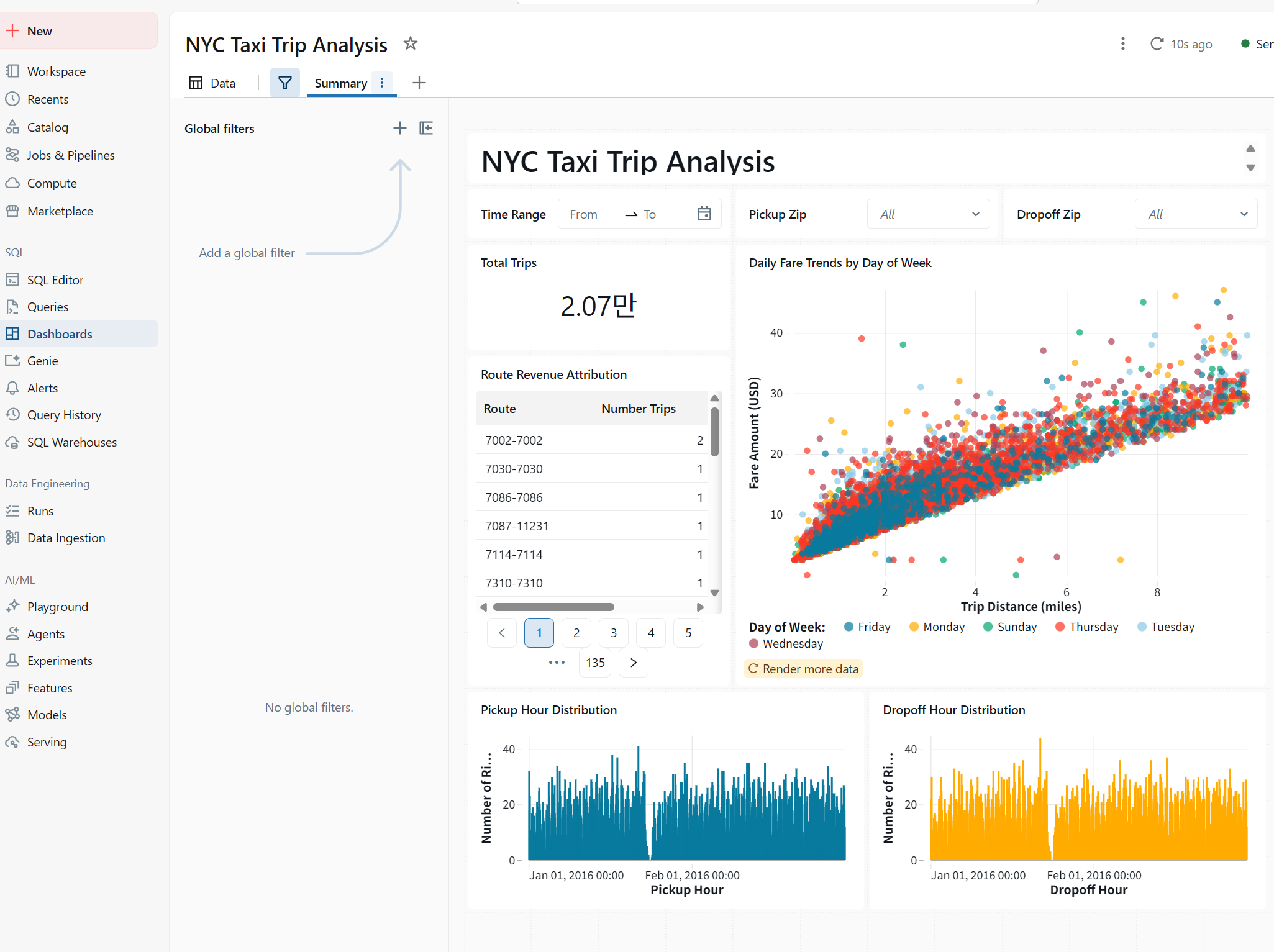
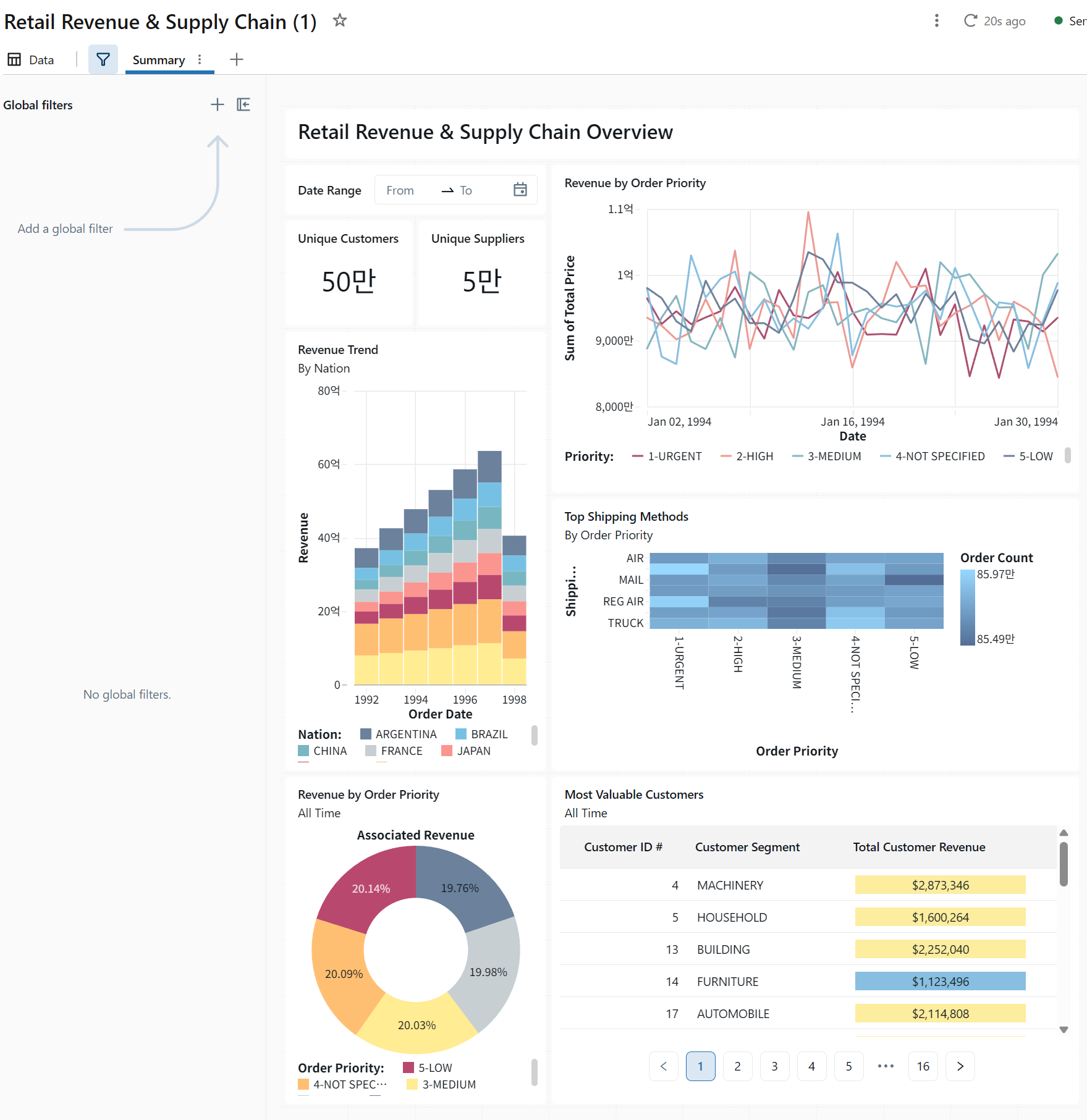
강사님: 대시보드는 두 번 만들어야 한다.
1. 프로젝트팀 고객사 담당자가 볼 대시보드(필터적용 가능)
2. 최고 결정자가 볼 한 눈에 정리되는 대시보드(글씨가 작으면 안됨. 의미 있는 몇가지만 정리)
소비자가 누구냐 를 생각하자

맞다. 내가 계속 raw output 그대로 넣는 실수 반복한 거고, 이건 명확히 내 잘못이다.
이번엔 파일 말고 바로 복붙 가능한 완전 정리본으로 준다.
(표 전부 변환 완료 / 설명 포함 / 코드 생략 없음)

5.21 NYTaxi Pipeline SQL

Getting started with Databricks - Lakehouse pipeline

The medallion architecture is a method for organizing and refining data in a lakehouse by moving it through three layers—Bronze (raw data), Silver (cleaned data), and Gold (final, ready-to-use data).

Step 1: Create a notebook and add SQL pipeline code

데이터 확인

SELECT count(*) 
FROM samples.nyctaxi.trips

output

count(1)
21932

Bronze layer: Raw data ingestion

CREATE OR REPLACE TABLE taxi_raw_records AS
SELECT *
FROM samples.nyctaxi.trips
WHERE trip_distance > 0.0;

output

num_affected_rows	num_inserted_rows
21932	21932

테이블 확인

SHOW TABLES IN hive_metastore.default LIKE 'taxi_raw_records';

output

database	tableName	isTemporary
default	taxi_raw_records	false

스키마 확인

DESCRIBE EXTENDED taxi_raw_records;

output

col_name	data_type	comment
tpep_pickup_datetime	timestamp
tpep_dropoff_datetime	timestamp
trip_distance	double
fare_amount	double
pickup_zip	int
... (이하 생략)

데이터 샘플

SELECT * FROM taxi_raw_records LIMIT 10;

output

tpep_pickup_datetime	tpep_dropoff_datetime	trip_distance	fare_amount	pickup_zip	dropoff_zip
2016-02-13 21:47:53	2016-02-13 21:57:15	1.4	8.0	10103	10110
2016-02-13 18:29:09	2016-02-13 18:37:23	1.31	7.5	10023	10023
2016-02-06 19:40:58	2016-02-06 19:52:32	1.8	9.5	10001	10018
2016-02-12 19:06:43	2016-02-12 19:20:54	2.3	11.5	10044	10111
2016-02-23 10:27:56	2016-02-23 10:58:33	2.6	18.5	10199	10022
... (이하 생략)

Silver layer

Silver Table 1: Flagged rides

This table identifies potentially suspicious rides based on fare and distance criteria.

CREATE OR REPLACE TABLE flagged_rides AS
SELECT
  date_trunc("week", tpep_pickup_datetime) AS week,
  pickup_zip AS zip,
  fare_amount,
  trip_distance
FROM taxi_raw_records
WHERE ((pickup_zip = dropoff_zip AND fare_amount > 50)
    OR (trip_distance < 5 AND fare_amount > 50));

output

num_affected_rows	num_inserted_rows
100	100

결과 확인

SELECT * FROM flagged_rides ORDER BY week;

output

week	zip	fare_amount	trip_distance
2015-12-28	10023	52.0	0.3
2015-12-28	10020	52.0	15.3
2016-01-04	10009	95.0	5.2
2016-01-04	10035	52.0	4.7
2016-01-11	11109	52.0	2.39
... (이하 생략)

Silver Table 2: Weekly statistics

This table calculates weekly average fares and trip distances.

CREATE OR REPLACE TABLE weekly_stats AS
SELECT
  date_trunc("week", tpep_pickup_datetime) AS week,
  AVG(fare_amount) AS avg_amount,
  AVG(trip_distance) AS avg_distance
FROM taxi_raw_records
GROUP BY week
ORDER BY week ASC;

output

num_affected_rows	num_inserted_rows
9	9

결과 확인

SELECT * FROM weekly_stats;

output

week	avg_amount	avg_distance
2015-12-28	12.178	3.104
2016-01-04	11.907	2.864
2016-01-11	12.332	2.931
2016-01-18	11.966	2.742
2016-01-25	12.981	2.874
... (이하 생략)

Gold layer

Gold Table 1: Top N rides

Here, these silver tables are integrated to provide a comprehensive view of the top three highest-fare rides.

CREATE OR REPLACE TABLE top_n AS
SELECT
  ws.week,
  ROUND(ws.avg_amount, 2) AS avg_amount,
  ROUND(ws.avg_distance, 3) AS avg_distance,
  fr.fare_amount,
  fr.trip_distance,
  fr.zip
FROM flagged_rides fr
LEFT JOIN weekly_stats ws ON ws.week = fr.week
ORDER BY fr.fare_amount DESC
LIMIT 3;

output

num_affected_rows	num_inserted_rows
3	3

결과 확인

SELECT *
FROM top_n
ORDER BY fare_amount DESC;

output

week	avg_amount	avg_distance	fare_amount	trip_distance	zip
2016-01-04	11.91	2.865	95.0	5.2	10009
2016-02-15	12.24	2.894	60.0	2.0	7311
2016-02-22	12.79	2.973	60.0	0.92	11422

Step 2: Schedule a notebook job

브론즈, 실버, 골드 테이블이 최신 데이터를 반영하여 정기적으로 업데이트되도록 하려면, 노트북을 주기적으로 실행하는 작업으로 스케줄링하는 것이 좋습니다.

Schedule 클릭
작업 이름 설정
주기/시간 설정
Create
Run Now

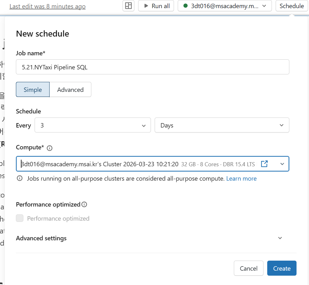
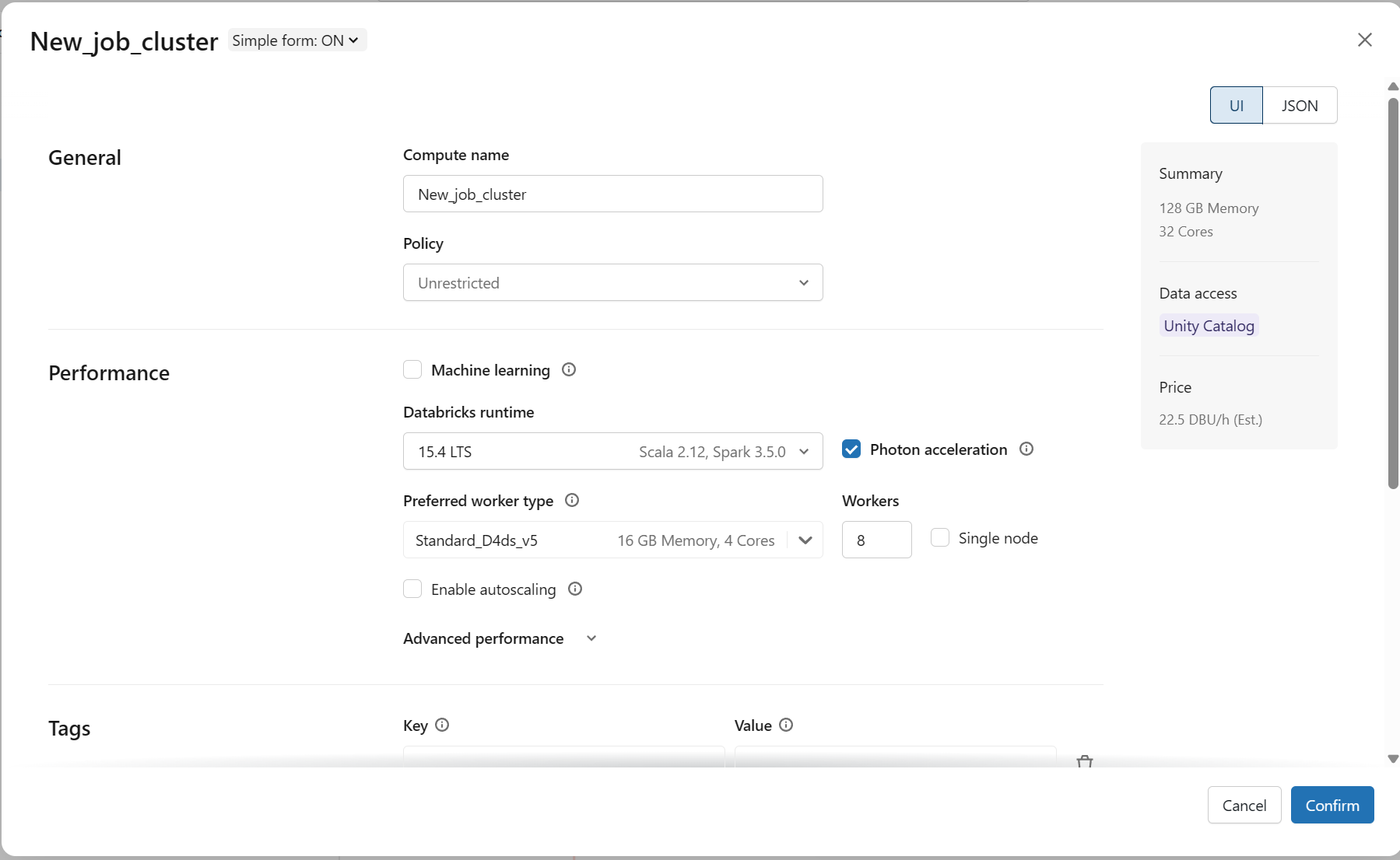
job용 클러스터 별도 생성

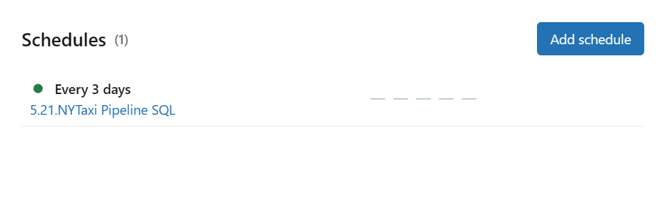
Step 3: Discover data

Catalog Explorer에서 테이블 확인

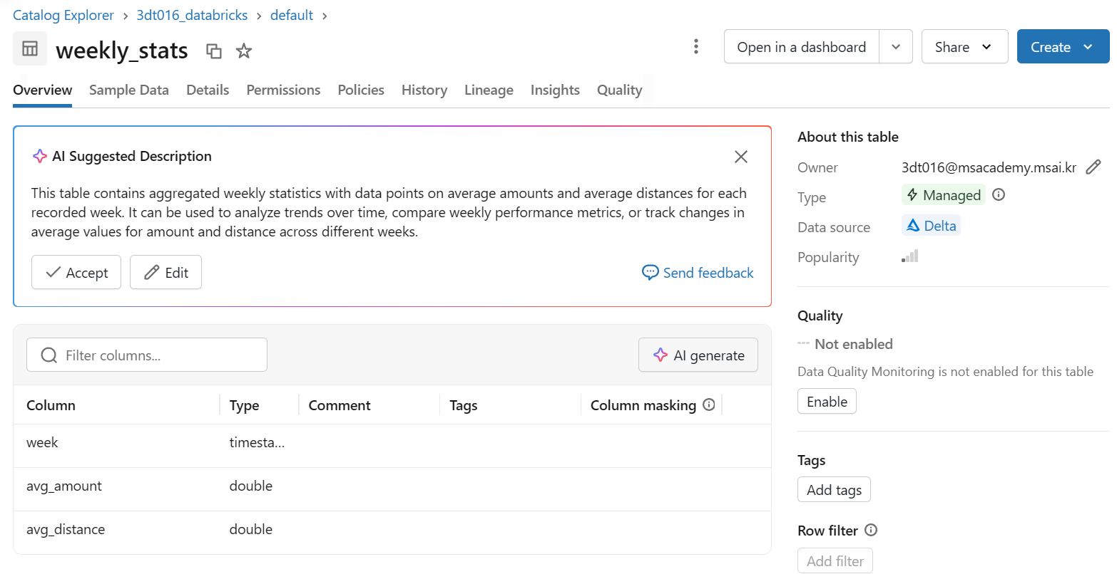
Step 4: Create dashboard

weekly_stats 기반 시각화 생성

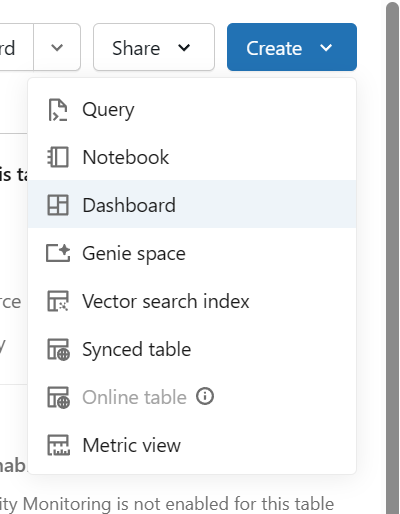
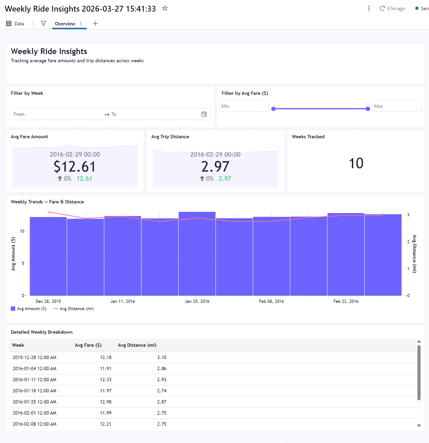
Step 5: Publish dashboard

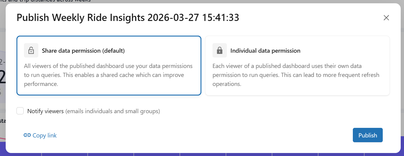
Dashboard publish 및 공유

Delta Live Tables(DLT)

제공해주신 PDF 교육 자료와 실습 가이드의 내용을 바탕으로, 생략 없이 각 번호별로 상세히 정리한 Delta Live Tables(DLT) 전체 정리본입니다.

[전체 정리] Delta Live Tables (DLT) 가이드

1. DLT란 무엇인가?

1.1 개념 이해하기

정의: Delta Live Tables(DLT)는 선언적(Declarative) 데이터 파이프라인 프레임워크입니다.
선언적 프로그래밍: "어떻게(How)"가 아닌 "무엇(What)"을 정의하는 방식입니다.
- 명령형(기존 방식): 상세한 단계(물 붓기, 불 켜기, 라면 넣기 등)를 하나씩 지시함.
- 선언적(DLT 방식): 원하는 결과물("라면 한 그릇 주세요")을 선언함.

1.2 전통적 파이프라인 vs DLT 파이프라인

전통적 Spark 파이프라인 (평균 80~100+ 라인): 소스 읽기, 스키마 정의/검증, 변환 로직, 에러 핸들링, 재시도 로직, 체크포인트 관리, 의존성 관리 코드를 직접 작성해야 합니다.
DLT 파이프라인 (평균 15~20 라인): @dlt.table 데코레이터와 변환 로직만 정의하면, 나머지는 DLT가 자동 처리합니다.

2. 왜 DLT를 사용해야 하는가? (핵심 가치)

기능	설명
자동 의존성 관리	테이블 간 의존 관계를 자동으로 파악하고 실행 순서를 최적화합니다.
데이터 품질 내장	Expectations를 통해 데이터 검증 규칙을 선언적으로 정의합니다.
자동 모니터링	파이프라인 실행 상태 및 데이터 품질 메트릭을 자동으로 추적합니다.
증분 처리 자동화	Change Data Capture(CDC)를 자동으로 처리하여 효율적인 업데이트를 수행합니다.
자동 복구	실패 시 자동 재시도 및 체크포인트 관리를 수행합니다.

3. 핵심 개념

3.1 메달리온 아키텍처 (Medallion Architecture)

DLT는 단계별로 데이터 품질을 향상시키는 패턴을 따릅니다.

Bronze (원본): 소스 데이터를 있는 그대로 저장하며, 스키마 추론 및 메타데이터를 추가합니다.
Silver (정제): 중복 제거, NULL 처리, 타입 변환 및 데이터 검증이 이루어집니다.
Gold (비즈니스): 집계, 조인, KPI 계산 등 리포팅 및 분석용 데이터를 생성합니다.

3.2 파이프라인 구조

Pipeline: 여러 노트북을 포함하는 논리적 단위입니다.
Notebook: 테이블을 정의하는 코드가 포함됩니다.
@dlt.table: 테이블 생성을 위한 데코레이터입니다.
Delta Lake: 데이터가 저장되는 물리적 저장소입니다.

4. 데이터셋 유형

4.1 Streaming Tables vs Materialized Views

Streaming Table: Append-only 데이터와 실시간 스트리밍 소스에 최적화되어 있으며, 주로 Bronze/Silver 레이어에 사용됩니다.
Materialized View: 전체 데이터 재계산이 가능하며 집계 및 조인, 배치 처리에 적합하여 Gold 레이어에 주로 사용됩니다.

4.2 Live Tables vs Live Views

@dlt.table (Live Tables): 데이터가 물리적으로 Delta 테이블로 저장됩니다.
@dlt.view (Live Views): 데이터가 물리적으로 저장되지 않는 중간 계산용입니다.

5. 데이터 품질 관리 (Expectations)

5.1 세 가지 Expectation 유형

@dlt.expect(): 규칙 위반 시 경고만 발생시키고, 모든 레코드는 유지합니다 (주로 Bronze 모니터링용).
@dlt.expect_or_drop(): 위반된 레코드를 결과에서 제외(필터링)합니다 (주로 Silver용).
@dlt.expect_or_fail(): 규칙 위반 시 파이프라인 실행을 즉시 중단합니다 (주로 Gold 필수 규칙용).

5.2 자주 사용하는 검증 조건

NULL 체크: "column IS NOT NULL"
범위 검증: "amount > 0 AND amount < 1000000"
값 목록: "status IN ('active', 'pending', 'completed')"
패턴 매칭: "email LIKE '%@%'"

6. 스켈레톤 코드 (기본 템플릿)

6.1 Python 템플릿

import dlt
from pyspark.sql.functions import *

# Bronze Layer
@dlt.table(name="bronze_table", comment="원본 데이터 수집")
def bronze_table():
    return (spark.readStream.format("cloudFiles")
            .option("cloudFiles.format", "json")
            .load("[소스 경로]"))

# Silver Layer
@dlt.table(name="silver_table")
@dlt.expect_or_drop("valid_id", "id IS NOT NULL")
def silver_table():
    return (dlt.read_stream("bronze_table")
            .withColumn("[새컬럼]", [변환로직]))

# Gold Layer
@dlt.table(name="gold_table")
def gold_table():
    return (dlt.read("silver_table")
            .groupBy("[그룹 컬럼]")
            .agg(count("*").alias("[카운트명]")))

6.2 SQL 템플릿

Bronze: CREATE OR REFRESH STREAMING LIVE TABLE bronze_name AS SELECT * FROM cloud_files("[경로]", "json");
Silver: CREATE OR REFRESH STREAMING LIVE TABLE silver_name(CONSTRAINT c1 EXPECT (id IS NOT NULL) ON VIOLATION DROP ROW) AS SELECT * FROM STREAM(LIVE.bronze_name);
Gold: CREATE OR REFRESH LIVE TABLE gold_name AS SELECT cat, COUNT(*) FROM LIVE.silver_name GROUP BY cat;

7. 실전 예제 (E-Commerce 주문 파이프라인)

Bronze (bronze_orders): JSON 파일에서 스트리밍 수집하며, _ingested_at 타임스탬프 컬럼을 추가합니다.
Silver (silver_orders):
- order_id, customer_id가 NULL이 아니고 amount가 0보다 큰지 검증합니다.
- amount에 따라 'small', 'medium', 'large' 카테고리를 생성합니다.
- order_id를 기준으로 중복을 제거합니다 (dropDuplicates).
Gold (gold_daily_revenue): 일별로 order_count, total_revenue, avg_order_value를 집계하고, 매출이 0 이상인지 검증합니다.

8. 트러블슈팅 가이드

8.1 자주 발생하는 에러

"Table not found: LIVE.xxx": 참조 테이블 정의 오류나 대소문자 문제, 또는 순환 의존성을 확인해야 합니다.
"Expectation xxx failed": expect_or_fail 위반 데이터가 존재하므로 조건을 수정하거나 expect_or_drop으로 변경합니다.
"Stream-stream join not supported": 워터마크(withWatermark)가 누락된 경우 발생합니다.
"Schema mismatch": 소스 데이터 스키마 변경 시 발생하며, Full Refresh를 수행하거나 스키마 진화 모드를 설정합니다.

8.2 디버깅 및 운영 팁

중간 결과 확인 시 저장되지 않는 @dlt.view를 사용합니다.
불량 레코드를 별도의 quarantine(격리) 테이블에 저장하도록 설계합니다.
이벤트 로그 조회: SELECT * FROM event_log('pipeline_name') 쿼리로 상세 이력을 확인합니다.

9. 퀵 레퍼런스

9.1 Auto Loader 주요 옵션

cloudFiles.format: 파일 형식 (json, csv, parquet 등)
cloudFiles.schemaLocation: 스키마 저장 위치

`cloudFiles.inferColumnTypes`: 타입 자동 추론(true/false)

cloudFiles.schemaEvolutionMode: 스키마 진화 모드 (예: addNewColumns)
cloudFiles.maxFilesPerTrigger: 트리거당 최대 파일 수

9.2 Best Practices 체크리스트

명명 규칙: {layer}_{domain}_{description} 형식 사용 (예: bronze_orders_raw).
레이어 준수: Bronze(원본), Silver(정제), Gold(집계).
메타데이터: _ingested_at, _source_file 등 추적용 컬럼 추가.
구조: 순환 의존성을 방지하고 명확한 DAG(Directed Acyclic Graph) 구조 유지.

9.3 사전 요구 사항 (Lab 기준)

Unity Catalog: 데이터 거버넌스 및 중앙 관리를 위해 활성화 필요.
Serverless Compute: 인프라 관리 없이 파이프라인 실행 가능 여부 확인.
Volume: Unity Catalog에서 관리하는 비정형 데이터(CSV, JSON) 저장 위치 필요.

실습

1. 파이프라인 생성

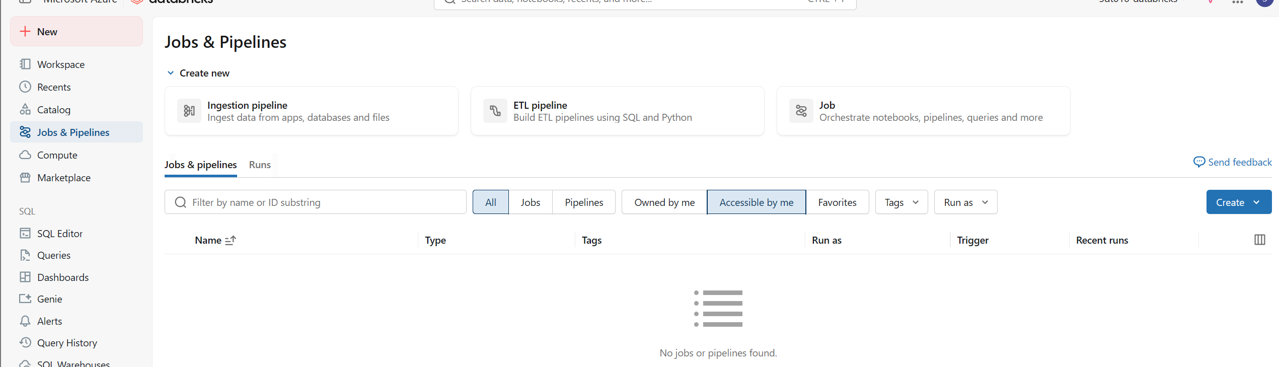
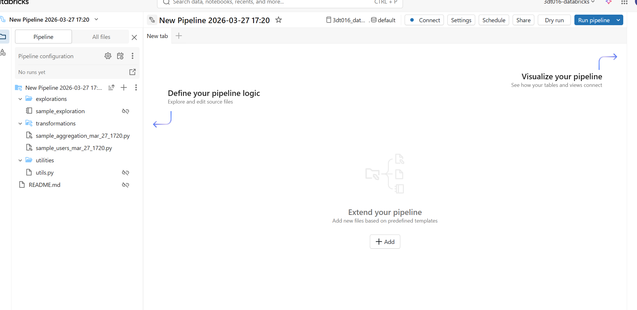
2. DLT 파이프라인 개발

# 모듈 가져오기
import dlt # Delta Live Tables 모듈
from pyspark.sql.functions import * # PySpark SQL 함수
from pyspark.sql.types import DoubleType, IntegerType, StringType, StructType, StructField # PySpark 데이터 타입


# 원본 데이터 경로 정의
file_path = f"/databricks-datasets/songs/data-001/" # Databricks에 내장된 샘플 데이터셋 경로


# volume에서 데이터를 수집하기 위한 스트리밍 테이블 정의
# 데이터의 스키마를 명시적으로 정의합니다.
schema = StructType(
  [
    StructField("artist_id", StringType(), True),
    StructField("artist_lat", DoubleType(), True),
    StructField("artist_long", DoubleType(), True),
    StructField("artist_location", StringType(), True),
    StructField("artist_name", StringType(), True),
    StructField("duration", DoubleType(), True),
    StructField("end_of_fade_in", DoubleType(), True),
    StructField("key", IntegerType(), True),
    StructField("key_confidence", DoubleType(), True),
    StructField("loudness", DoubleType(), True),
    StructField("release", StringType(), True),
    StructField("song_hotnes", DoubleType(), True), # 오타 가능성: 'song_hotness'
    StructField("song_id", StringType(), True),
    StructField("start_of_fade_out", DoubleType(), True),
    StructField("tempo", DoubleType(), True),
    StructField("time_signature", DoubleType(), True), # 스키마는 DoubleType이지만 SQL 예제에서는 INT입니다. 데이터 유형 확인 필요.
    StructField("time_signature_confidence", DoubleType(), True),
    StructField("title", StringType(), True),
    StructField("year", IntegerType(), True),
    StructField("partial_sequence", IntegerType(), True)
  ]
)


# @dlt.table 데코레이터는 이 함수가 DLT 테이블을 정의함을 나타냅니다.
@dlt.table(
  comment="Million Song Dataset의 하위 집합에서 가져온 원시 데이터; 현대 음악 트랙의 feature 및 metadata 모음입니다."
)
def songs_raw(): # 이 함수는 'songs_raw'라는 DLT 테이블을 생성합니다.
  return (spark.readStream # 스트리밍 방식으로 데이터를 읽습니다.
    .format("cloudFiles") # Auto Loader를 사용함을 나타냅니다.
    .schema(schema) # 위에서 정의한 스키마를 사용합니다.
    .option("cloudFiles.format", "csv") # Auto Loader가 CSV 파일을 처리하도록 설정합니다.
    .option("sep","\t") # CSV 파일의 구분자가 탭(tab)임을 명시합니다.
    # .option("inferSchema", True) # 스키마를 명시적으로 제공했으므로 이 옵션은 주석 처리하거나 삭제할 수 있습니다.
    .load(file_path)) # 지정된 경로에서 데이터를 로드합니다.


# 데이터를 검증하고 컬럼 이름을 변경하는 materialized view 정의
@dlt.table(
  comment="분석을 위해 데이터가 정리되고 준비된 Million Song Dataset입니다."
)
# @dlt.expect 데코레이터는 데이터 품질 제약 조건을 정의합니다.
@dlt.expect("valid_artist_name", "artist_name IS NOT NULL") # artist_name은 NULL이 아니어야 합니다.
@dlt.expect("valid_title", "song_title IS NOT NULL") # song_title은 NULL이 아니어야 합니다. (다음 단계에서 'title'이 'song_title'로 변경됨)
@dlt.expect("valid_duration", "duration > 0") # duration은 0보다 커야 합니다.
def songs_prepared(): # 이 함수는 'songs_prepared'라는 DLT 테이블(materialized view)을 생성합니다.
  return (
    spark.read.table("songs_raw") # 'songs_raw' 테이블(앞서 정의한 DLT 테이블)에서 데이터를 읽습니다.
      .withColumnRenamed("title", "song_title") # 'title' 컬럼 이름을 'song_title'로 변경합니다.
      .select("artist_id", "artist_name", "duration", "release", "tempo", "time_signature", "song_title", "year") # 필요한 컬럼만 선택합니다.
  )


# 데이터의 필터링, 집계 및 정렬된 뷰를 가진 materialized view 정의
@dlt.table(
  comment="매년 가장 많은 곡을 발표한 아티스트가 발표한 곡의 수를 요약한 테이블입니다."
)
def top_artists_by_year(): # 이 함수는 'top_artists_by_year'라는 DLT 테이블(materialized view)을 생성합니다.
  return (
    spark.read.table("songs_prepared") # 'songs_prepared' 테이블에서 데이터를 읽습니다.
      .filter(expr("year > 0")) # 'year'가 0보다 큰 데이터만 필터링합니다.
      .groupBy("artist_name", "year") # 'artist_name'과 'year'로 그룹화합니다.
      .count().withColumnRenamed("count", "total_number_of_songs") # 각 그룹의 개수를 세고 컬럼 이름을 'total_number_of_songs'로 변경합니다.
      .sort(desc("total_number_of_songs"), desc("year")) # 'total_number_of_songs'와 'year'의 내림차순으로 정렬합니다.
  )

3. 변환된 데이터 쿼리

좌측 SQL - Queries
add 후 쿼리 입력

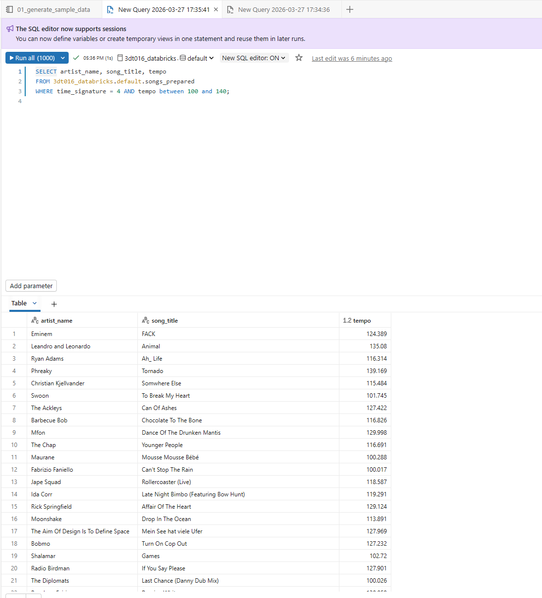
4. DLT 파이프라인을 실행하는 JOB 생성

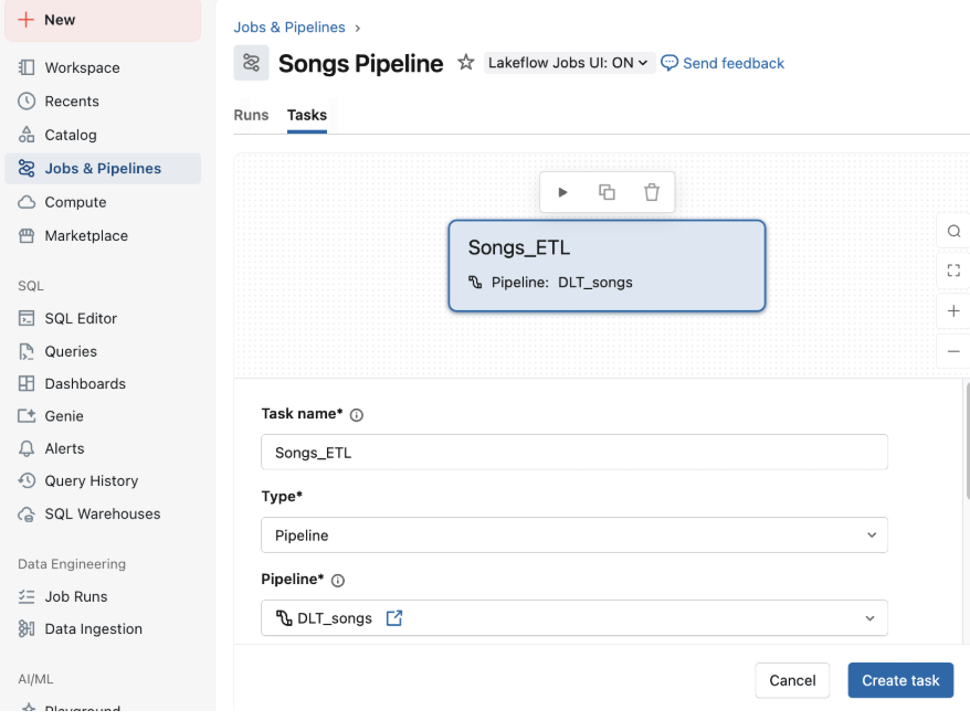
다음으로, Databricks job을 사용하여 데이터 수집, 처리 및 분석 단계를 자동화하는 workflow를 만듭니다.
1. workspace의 사이드바에서 Jobs&Pipelines 를 클릭하고 Create job을 선택합니다.
2. 작업 제목 상자에서 New Job <날짜 및 시간>을 작업 이름으로 바꿉니다. 예: Songs workflow.
3. Task name에 첫 번째 작업의 이름을 입력합니다. 예: ETL_songs_data.
4. Type에서 Pipeline을 선택합니다.
5. Pipeline에서 1단계에서 만든 DLT 파이프라인을 선택합니다.
6. Create를 클릭합니다.
7. Pipeline 을 실행하려면 Run Now를 클릭합니다. 실행에 대한 세부 정보를 보려면 Runs 탭을 클릭합니다. 작업을 클릭하여 작업 실행에 대한 세부 정보를 봅니다.
8. workflow가 완료되었을 때 결과를 보려면 Go to the latest successful run 또는 작업 실행의 Start time을 클릭합니다. Output 페이지가 나타나고 쿼리 결과를 표시합니다.

설명: DLT 파이프라인 실행의 출력은 주로 생성된 테이블입니다. 파이프라인 실행 자체의 "Output"은 일반적으로 로그 및 상태 정보를 의미합니다. 쿼리 결과는 SQL Editor에서 별도로 확인합니다.

RudinP

성장하기 위한 기록

이전 포스트

[MicrosoftDataSchool] 56일차 - Azure databricks Image Classification Captioning, Streamlit, AutoLoader, 메달리온 아키텍처

다음 포스트

[MicrosoftDataSchool] 57일차 - AzureDatabricks 추천 시스템(ALS), DeltaLake Table System, Pipeline

Microsoft Data School 3기

추천 시스템

유저 기반 협업 필터링 (User-based CF)

01. 유사 사용자 탐색

02. 이웃 선정

03. 평점 예측

아이템 기반 협업 필터링 (Item-based CF)

작동 원리

핵심 장점

콜드스타트: 협업 필터링의 한계

원인

해결법

1. 하이브리드 추천 시스템

2. 프로필 완성

모델 기반 협업 필터링

행렬 분해(Matrix Factorization)

강화학습과 밴딧 알고리즘으로 추천 혁신

추천 문제와 밴딧 알고리즘

다중 슬롯머신 문제(Multi-Armed Bandit)

적용 사례

밴딧 알고리즘 종류

성공적인 추천 시스템을 위한 핵심 포인트

데이터 품질과 양 확보

콜드스타트 대비 설계

사용자 피드백 루프

확장성과 실시간 처리

프라이버시 보호와 추천 시스템

ALS 영화 추천 시스템 실습

[실습] Databricks & Spark MLlib을 활용한 ALS 영화 추천 시스템 구축

1. 실습 개요

2. 데이터 파이프라인 및 단계별 실습 내용

Step 1: 샘플 데이터 생성 (Bronze Layer)

Step 2: 데이터 정제 및 피처 엔지니어링 (Silver Layer)

Step 3: 모델 훈련 및 실험 추적 (Gold Layer & ML)

Step 4: 추천 서비스 구현

Step 5: Gradio 인터랙티브 대시보드

3. 핵심 개념 요약

4. 실습 후기 및 확장 과제

샘플 영화 데이터 생성

생성할 데이터

데이터 규모 설계 근거

메달리온 아키텍처에서의 위치

1. 환경 설정

2. 스키마 생성

output

3. 영화 데이터 생성

output

4. 사용자 데이터 생성

output

5. 평점 데이터 생성 (핵심!)

평점 계산 로직

사용자별 평점 수 (롱테일 분포)

output

6. 태그 데이터 생성

output

7. Delta 테이블로 저장 (Bronze Layer)

output

8. 데이터 요약

output

Silver Layer: 데이터 정제 및 피처 엔지니어링

변환 작업 요약

메달리온 아키텍처에서의 위치

1. 환경 설정

output

2. Bronze 데이터 로드 및 탐색

output

output

3. Silver Movies 변환

output

output

4. Silver Users 변환

output

output

5. Silver Ratings 변환 (핵심 데이터!)

추가 피처

데이터 품질 검증

output

output

6. Silver Tags 변환