from datetime import datetime
from pytz import timezone
def tmstmp(): return datetime.now(timezone('Asia/Seoul')).strftime('%Y-%m-%d-%H:%M:%S')
def tmstmp_ymd(): return datetime.now(timezone('Asia/Seoul')).strftime('%Y%m%d')
def tmstmp_hm(): return datetime.now(timezone('Asia/Seoul')).strftime('%H%M')
from tensorflow.keras import datasets, layers, models
import matplotlib.pyplot as plt
import numpy as np
import torch
from torch.utils.data import Dataset
import torch.nn as nn
import torch.nn.functional as F
import torch.optim as optimDataset
* CIFAR-10 : 32×32 컬러 이미지 6,000개 (훈련 5,000 / 테스트 1,000)cifar10 = datasets.cifar10
(train_images, train_labels), (test_images, test_labels) = cifar10.load_data()
class_names = ['airplane', 'automobile', 'bird', 'cat', 'deer', 'dog', 'frog', 'horse', 'ship', 'truck']
class_dict = {i:x for i,x in enumerate(class_names)}
train_images.shape, train_labels.shape, test_images.shape, test_labels.shape
#((50000, 32, 32, 3), (50000, 1), (10000, 32, 32, 3), (10000, 1))- 50,000개 train 10,000개 test
- 32×32 이미지, 3개(RGB) 채널(channel = depth)
plt.imshow(train_images[1])
print(class_dict[train_labels[1][0]])
#truck
* data shape : (N, C=channel, H, W)
train_images = np.transpose(train_images, (0, 3, 1, 2))
test_images = np.transpose(test_images, (0, 3, 1, 2))
train_images.shape, test_images.shape
#((50000, 3, 32, 32), (10000, 3, 32, 32))- output label one-hot encoding
train_labels_encod = np.eye(10)[train_labels.flatten().astype(int)]
test_labels_encod = np.eye(10)[test_labels.flatten().astype(int)]- batch 생성해주는 DataLoader 활용 위해서는 __getitem__, __len__속성 필요
class Dataset(Dataset):
    def __init__(self, X, y):
        self.X = torch.tensor(X).float()
        self.y = torch.tensor(y).float()
    def __getitem__(self, i):
        return (self.X[i], self.y[i])
    def __len__(self):
        return (len(self.X))
# trains = Dataset(train_images, train_labels_encod)
# tests = Dataset(test_images, test_labels_encod)
trains = Dataset(train_images, train_labels)
tests = Dataset(test_images, test_labels)- train/valdation split > 4:1
tra, val = torch.utils.data.random_split(trains, [40000, 10000])modeling
- pytorch based neural network model 기본구조
class Model(nn.Module):  # Base class(nn.Module) 상속 필수
    def __init__(self):  # model 설계 : layer 설계 & parameter 설계
        super(Model, self).__init__()
        layer1 = nn.linear(input shape, output1 shape, parameters)
        layer2 = nn.conv1d(output1 shape, output2 shape, parameters)
        ....
        layer = nn.Dropout(output shape, final_output shape, parameters)
    def forward(self, input_x):
        output1 = layer1(input_x)
        output2 = layer2(output1)
        ....
        final_output = layer(output)
        return x
class Model(nn.Module):
def __init__(self):
super(Model, self).__init__()
# 테스트를 위해 간소한 모델 설계
self.layer1 = nn.Conv2d(in_channels = 3, out_channels = 3, kernel_size = (8,8), stride=8) # 3(C)×32×32 input > 3(C)×4×4 output
self.layer2 = nn.Conv2d(in_channels = 3, out_channels = 3, kernel_size = (4,4)) # 3(C)×4×4 input > 3(C)×1×1 output
self.linear = nn.Linear(3,10) # 3(C)×1×1 output > 10 classification by linear regression
def forward(self, input_x):
x = self.layer1(input_x)
x = self.layer2(x).squeeze()
x = self.linear(x)
return x
model = Model()training
- pytorch based neural network training 기본구조
# 데이터셋 shuffle batch 구성(torch 제공)
train_batches = torch.utils.data.DataLoader(trains, batch_size=batch_size, shuffle=True)
test_batches = torch.utils.data.DataLoader(tests, batch_size=batch_size, shuffle=True)
for epoch in range(num_epoch):          # num_epochs 수 만큼 반복
    model.train() # 모델 학습 (평가 : model.eval())
    for i_batch, batch in enumerate(train_batches):  # batch 마다 가중치 update
        X, y = batches[0], batches[1]
        optimizer.zero_grad()         # 기울기 초기화
        out = model(X)                # 예측값
        loss = loss_func(out, y)      # loss 계산
        loss.backward()               # 역전파(back propagation) : 파라미터들의 에러에 대한 변화도를 계산하여 누적
        optimizer.step()              # loss가 최소가 될 수 있도록 가중치 수정
Q) epoch마다 train/validation split을 수행하는 알고리즘
A) epoch 마다 다른 train/validation set 사용
    > validation set에 이전 epoch에서 학습한 데이터가 포함됨
1. training hyperparameter
a. num_epoch = Number of Epochs : the number times of iterate over the dataset
모델 수행 횟수
1 < epoch < ∞
b. batch_size = Batch size : the number of data samples propagated through the network before the parameters are updated
내부 모델 파라미터 업데이트 전 샘플 수
1 < batch_size < 데이터 전체 샘플 수
[examples] 200 samples, batch_size=5, epoch=100
{batch_size = 5} ⇒ 40 chunks of 5 samples > weights update 40 times (for 1 traning)
{epoch = 100} ⇒ iterate model 100 times (traning 100 times)
> weights update 40(batch)×100(epoch)=40,000 timesTest
batch_size = 100 # 100개 샘플로 구성된 400개 batch
print_log_interval = int((len(trains)/batch_size)/10)
num_epoch = 10 # training 10번 반복
loss_func = torch.nn.CrossEntropyLoss() # multiclass classification을 위한 loss function
optimizer = optim.Adam(model.parameters(), lr=0.0005)
tra_batches = torch.utils.data.DataLoader(tra, batch_size=batch_size, shuffle=True) # train set shuffle batch 생성
val_batches = torch.utils.data.DataLoader(val, batch_size=batch_size, shuffle=True) # validation set shuffle batch 생성
ACC = 0 # 초기 정확도
model_name = f"./test_{tmstmp_hm}.pth"
for epoch in range(num_epoch):
    train_loss = 0
    model.train() # training model
    for i_batch, batch in enumerate(tra_batches):  # batch 마다 가중치 update
        X, y = batch[0], batch[1]
        optimizer.zero_grad() # loss.backward() > optimizer.step() 시 gradient가 누적되기 때문에 초기화 필요
        out = model(X) # 예측값
        loss = loss_func(out, y.long().squeeze()) # loss 계산
        # CrossEntropyLoss > target should be of type torch.long
        loss.backward()
        optimizer.step()
        train_loss += loss
    test_loss = 0
    model.eval() # evaluating model
    ACC1 = 0 ; ACC2 = 0 ; PREC1 = 0 ; PREC2 = 0 # 성능 지표를 위한 초기값
    for i_batch, batch in enumerate(val_batches):
        with torch.no_grad(): # 메모리 사용량 감소, 연산 속도 향상
            X, y = batch[0], batch[1]
            out = model(X)                  # 예측값
            loss = loss_func(out, y.long().squeeze())
            # 누적 성능 확인용 수치 ACC=(TP+TN)/Total
            avgloss = loss/len(y)
            test_loss += avgloss             # 평균loss
            ACC1 += len(y)
            ACC2 += sum(out.argmax(dim=1).unsqueeze(dim=1) == y).item()
    print(f"epoch #{epoch+1} validation\tAcc : {ACC2/ACC1}\tTest Loss : {test_loss/(i_batch+1)}")
    # model 성능(ACC기준) 개선시 저장
    if ACC < (ACC2/ACC1):
        torch.save(model.state_dict(),model_name)
#epoch #1 validation	Acc : 0.108	Test Loss : 0.02898138202726841
#epoch #2 validation	Acc : 0.1171	Test Loss : 0.02440040558576584
#epoch #3 validation	Acc : 0.1413	Test Loss : 0.023326747119426727
#epoch #4 validation	Acc : 0.1654	Test Loss : 0.022504761815071106
#epoch #5 validation	Acc : 0.1826	Test Loss : 0.021916143596172333
#epoch #6 validation	Acc : 0.1847	Test Loss : 0.021501503884792328
#epoch #7 validation	Acc : 0.2185	Test Loss : 0.02101852372288704
#epoch #8 validation	Acc : 0.2289	Test Loss : 0.020669851452112198
#epoch #9 validation	Acc : 0.2409	Test Loss : 0.02021060697734356
#epoch #10 validation	Acc : 0.2555	Test Loss : 0.020031414926052094
2. loss function
a. Regression > MSE(Mean Square Error), MAE(Mean Absolute Error), RMES(Root Mean Square Eror)
b. Classificatoin > entropy based : Binary Crossentropy, Categorical Crossentropy, Sparse Categorical Erossentropy
3. optimizer
a. Gradient Descent(경사 하강법) = Batch Gradient Descent
* 전체 data에 대하여 loss를 계산하여 loss 값이 최소인 weight를 찾음
* [장] 전체 data에 대해 gradient를 계산하기 때문에 안정적으로 optimal로 수렴
       업데이트 자체는 한번에 이루어지기 때문에 계산 횟수는 적음
* [단] 한 스텝에 전체 데이터 사용으로 학습이 오래걸림(계산 오래걸림)
       local minima에 수렴 시 빠져나오기 어려움
a-1. SGD(Stochastic Gradient Descent, 확률적 경사 하강법)
* 추출한 한개의 sample data에 대하여 Gradient Descent 알고리즘 적용
* local optimal에 빠질 리스크 적음, 1 step에 걸리는 시간이 매우 짧음
* global optimal 찾지 못할 수 있음, 병렬처리가 어려움
b. MSGD(Mini-Batch Stochastic Gradient Descent)
* data sample(mini-batch)이 전체 data와 유사한 gradient를 가진다는 가정 하에 sample에 대한 loss를 계산하여 보정
* 단점 : oscilation 현상으로 global minima(optimal)을 찾지 못하고 local minima로 수렴할 수 있음
c. Momentum
* gradient에 이전 step 방향(관성)과 를 더해 현재 학습 방향과 크기 결정
* local minimum을 빠져나올 수 있음 (SGD의 oscilation 현상 해결)
d. Adagrad(Adaptive Gradient)
* parameter 변화도에 반비례하는 gradient를 줌(변화가 큰 변수는 step size를 작게, 변화가 작은 변수는 step size를 크게)
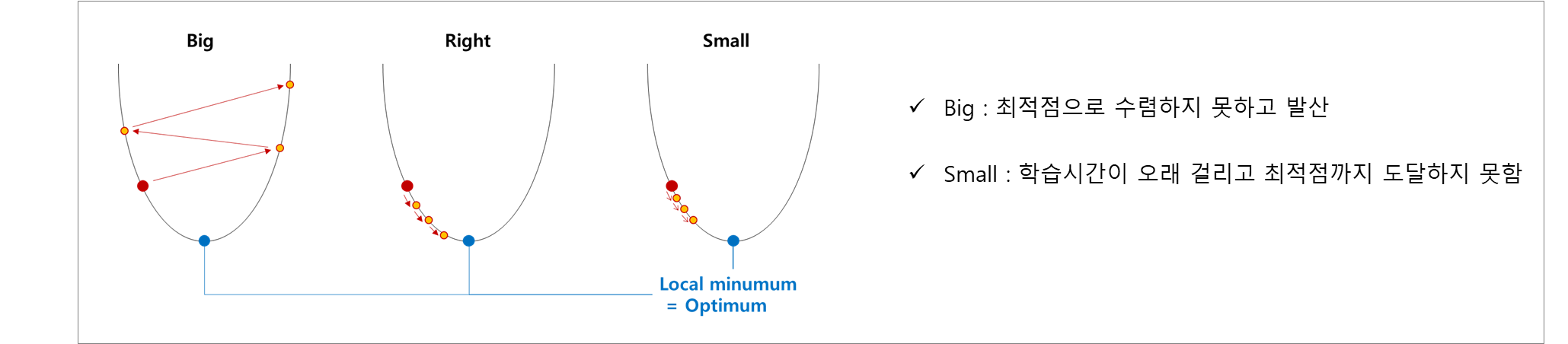
* 학습이 오래 진행될 경우 많이 변화한 변수들의 학습이 제대로 이루어지지 않음 * lr = Learning Rate : how much to update models parameters at each batch/epoch
Gradient Descent 알고리즘에서 Optimum(loss가 최소인 점)에 도달하기 위한 Step size
현재 시점 weight의 gradient×Learning Rate만큼 weight가 수정됨 (업데이트 정도)
Gradient Descent Algorithm(경사하강법 알고리즘) : Weight(t) = Weight(t-1) - Learning Rate × Gradient(t-1)