색 공간 (Color Space)

색공간이란?

색을 표현하기 위한 다양한 방법을 의미, 여러 방법이 있으며 각각 목적에 따라 설계되어 고유한 특성을 가진다.

• RGB: 일반적으로 디지털 이미지에서 사용되는 색 공간.
• HSV: 색상(Hue), 채도(Saturation), 명도(Value)로 구성된 색 공간.
• LAB: 인간의 시각 체계와 유사한 방식으로 색 차이를 표현하는 색 공간.
• Grayscale: 흑백 이미지를 위한 색 공간.

RGB (Red, Green, Blue)

RGB는 디지털 이미지에서 가장 널리 사용되는 색 공간입니다.

• 구성: 빨강(Red), 초록(Green), 파랑(Blue)의 세 가지 색상 채널로 구성됩니다.
• 특징:
  • 직관적이며, 대부분의 디스플레이와 카메라에서 기본적으로 사용됩니다.
  • 각 채널은 0~255 사이의 값으로 표현되며, 이를 조합하여 1677만 가지 색상을 표현할 수 있습니다.
    

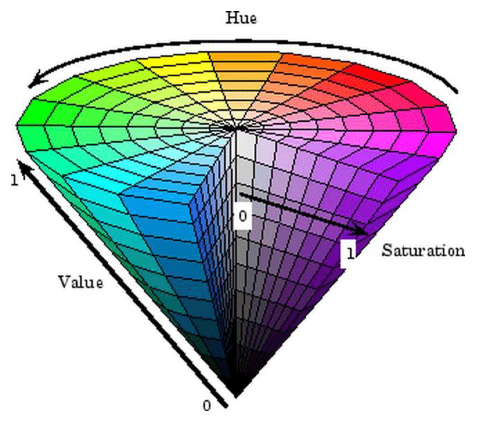
HSV (Hue, Saturation, Value)

HSV는 색상의 종류, 강도, 밝기를 분리하여 표현하는 색 공간입니다.

• 구성: 색상(Hue), 채도(Saturation), 명도(Value)로 구성됩니다.
• 특징:
  • Hue: 색상의 종류를 나타내며, 0~360도의 각도로 표현됩니다 (빨강, 주황, 노랑 등).
  • Saturation: 색상의 강도를 나타내며, 0~100%의 범위로 표현됩니다 (100%는 가장 진한 색).
  • Value: 색상의 밝기를 나타내며, 0~100%의 범위로 표현됩니다.
    

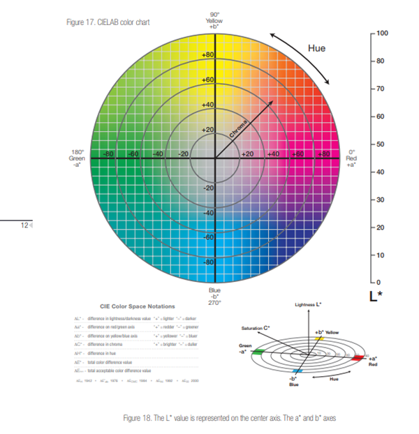
LAB

LAB 색 공간은 인간의 시각 체계를 반영하여 설계되었습니다.

• 구성: L은 밝기, A와 B는 색상을 표현합니다.
• 특징:
  • L 채널은 밝기를 나타내며, A와 B 채널은 색상을 나타냅니다.
  • LAB 색 공간은 색 차이를 일관되게 표현할 수 있어 색상 처리에 적합합니다.
    

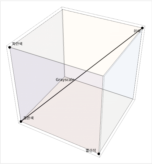
Grayscale

Grayscale은 흑백 이미지를 표현하기 위한 색 공간입니다.

• 특징:
  • 색상 정보 없이 밝기 정보만으로 이미지를 표현합니다.
  • 각 픽셀은 0(검은색)에서 255(흰색) 사이의 값으로 표현됩니다.
    

---

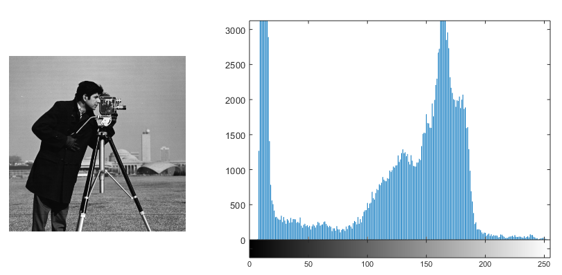
이미지 히스토그램 (Image Histogram)

히스토그램이란?

데이터의 분포를 그래프 형태로 표현헌 것으로, 이미지 처리에서의 히스토그램은 주로 이미지의 밝기 값을 나타내며, 각 밝기 값에 해당하는 픽셀의 수를 세로축으로 표시한다.

• 이미지의 명암 분포를 쉽게 파악할 수 있음

• 이미지의 전반적인 대비와 밝기 수준을 평가하거나 조정하는데 도움을 줌
  

• $x$축 : 이미지의 밝기(0~255)

• $y$축 : 등장 빈도

  응용

  히스토그램 평활화 (Histogram Equalization)

  픽셀의 값을 0부터 255까지의 누적치가 전체 영역에서 고르게 분포되도록 만드는 기법으로 이미지가 전체적으로 어둡거나 고루 밝아 특징이 눈에 띄지 않거나 분리가 어려울 때 자주 쓰입니다.

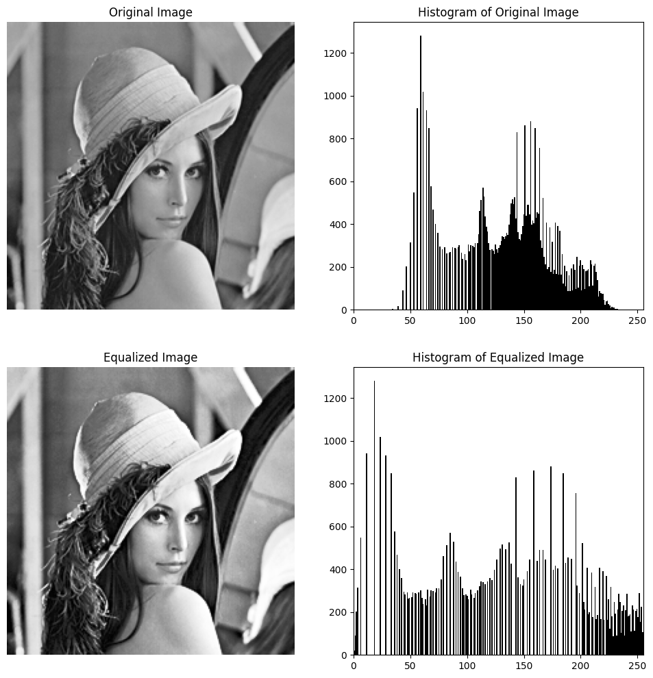  위 이미지를 보시면 모자의 그림자와 여성 피부와의 대비가 커진 것을 확인 할 수 있습니다. 즉, 어두운 것은 더욱 어둡게, 밝은 것은 더욱 밝아졌습니다. 이는 원본 이미지의 분포가 중간밝기에 밀집되었기 때문입니다.

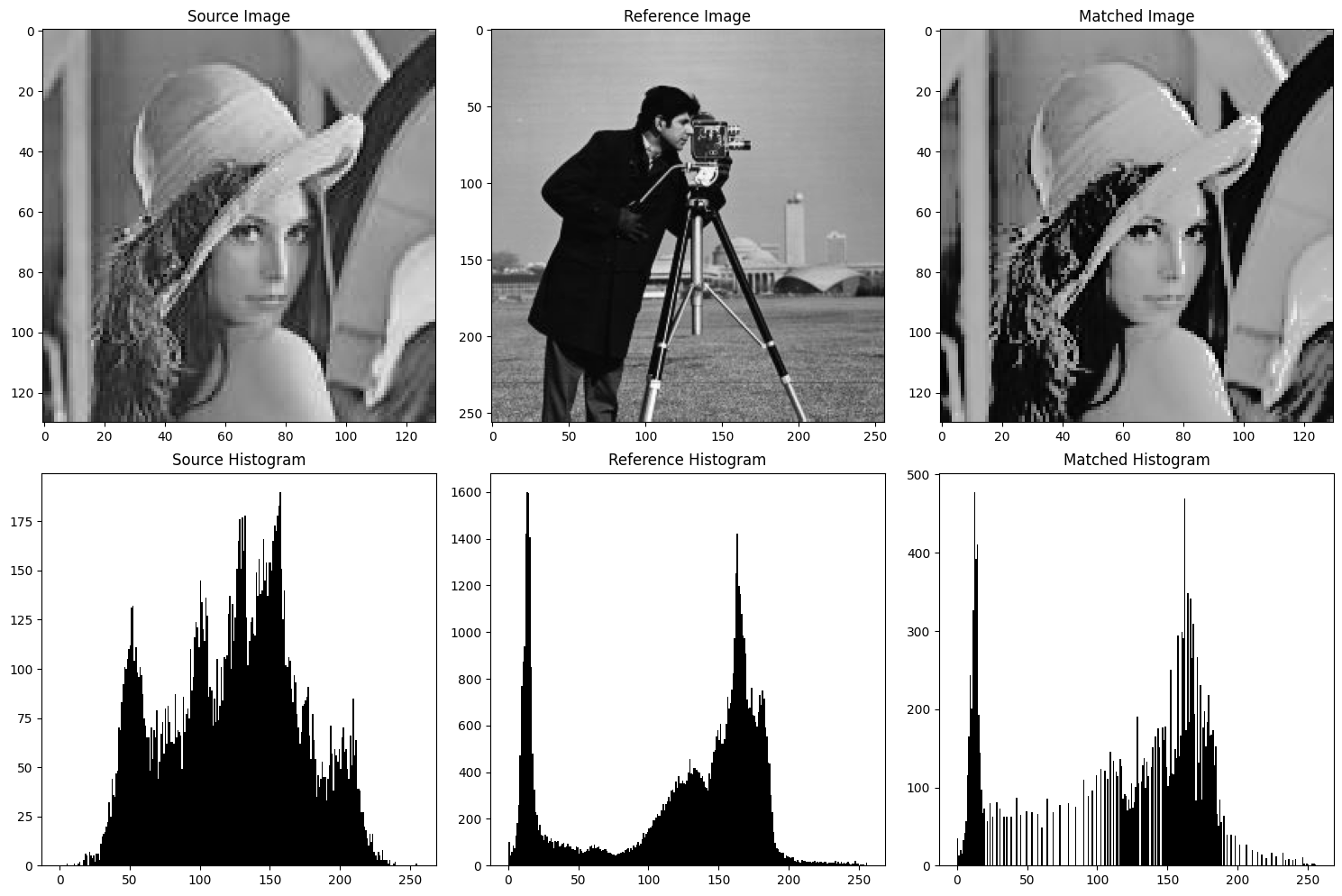
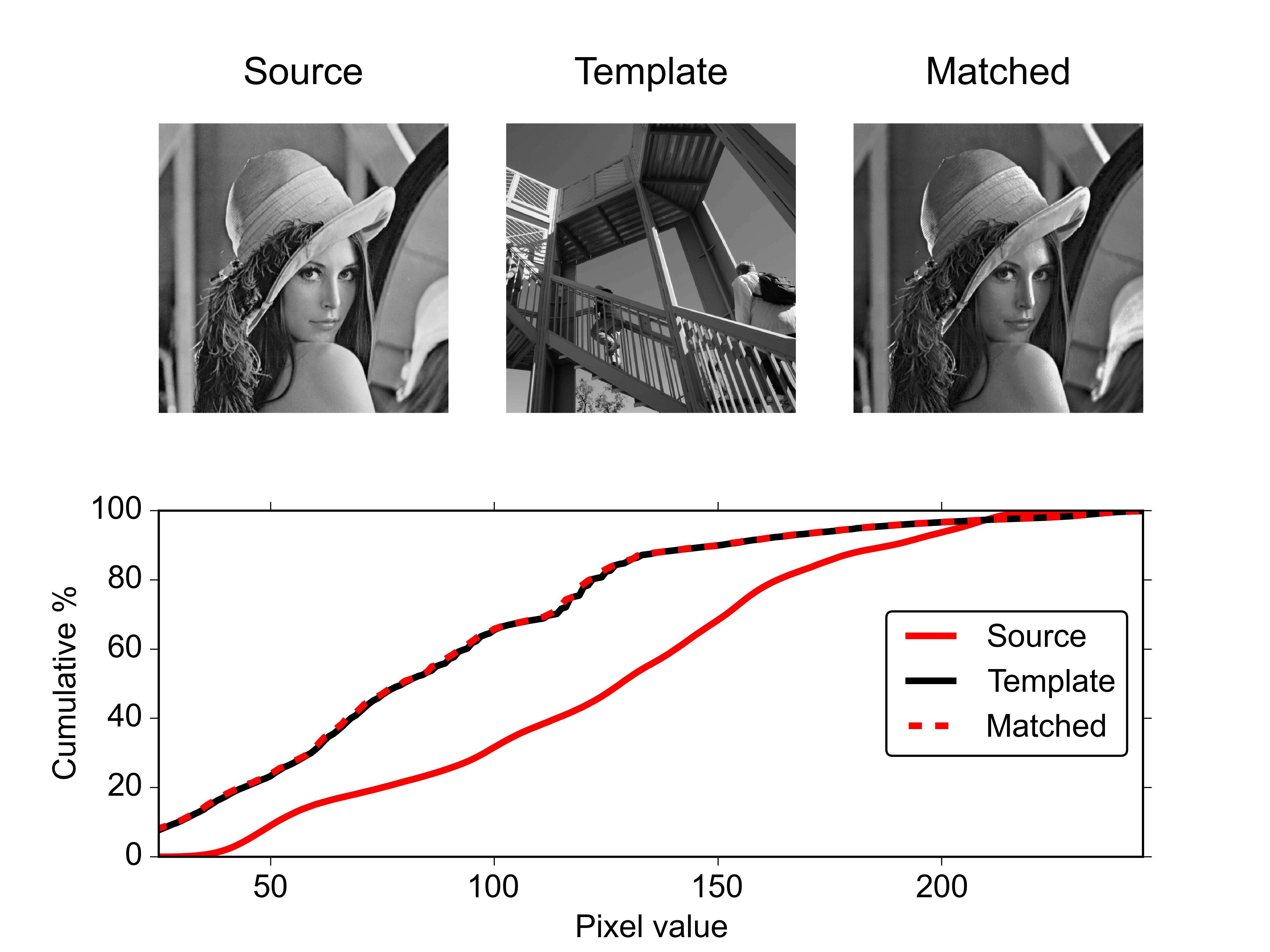
  히스토그램 매칭 (Histogram Matching)

  히스토그램 매칭은 한 이미지의 히스토그램을 다른 이미지의 히스토그램과 유사하게 조정하는 과정입니다. 다양한 환경에서 촬영된 이미지의 밝기 및 대비를 일관되게 만드는데 사용할 수 있습니다.

  

---

이미지 변환 (Image Transformations)

이미지 변환이란?

이미지 변환은 이미지의 픽셀 위치나 값을 변경하여 원본 이미지를 다른 형태나 모양으로 변환하는 것을 의미합니다. 기하학적 구조를 변경하거나 이미지의 밝기, 색상을 조절할 수 있으며 이미지 편집, 개선, 분석 등 다양한 처리 작업에 사용됩니다.

기하학적 변환 (Geometric Transformations)

기하학적 변환은 이미지의 모양이나 위치를 변환하는 것입니다.

- 스케일링 (Scaling)

• 이미지의 크기를 확대 또는 축소하는 변환입니다.
• 보간법(Interpolation)을 사용하여 새로운 픽셀 값을 결정합니다.

- 회전 및 이동

• 회전은 이미지를 중심점을 기준으로 특정 각도로 회전시키는 변환입니다.
• 이동은 이미지를 x, y 방향으로 특정 거리만큼 이동시키는 변환입니다.

- 아핀 변환

• 스케일링, 회전, 이동 등의 기본 변환을 조합하여 수행하는 변환입니다.
• 3개의 점을 원본 이미지와 대상 이미지 간에 매핑하여 변환 매트릭스를 생성하고, 이를 사용하여 이미지를 변환합니다.

Python Example

💻 예제

import cv2
import numpy as np
import matplotlib.pyplot as plt
# 포인트에 원을 그려주는 함수
def draw_points(image, points, color, border_color, size=3):
    for point in points:
        center = (int(point[0]), int(point[1]))
        cv2.circle(image, center, size, border_color, -1)
        cv2.circle(image, center, size-1, color, -1)

# 이미지 불러오기
img = cv2.imread('lenna.jpg')
img = cv2.cvtColor(img, cv2.COLOR_BGR2RGB)

# 아핀 변환
rows, cols, ch = img.shape
src_points = np.float32([[0, 0], [cols - 1, 0], [0, rows - 1]])
dst_points = np.float32([[cols * 0.1, rows * 0.1], [cols * 0.9, rows * 0.2], [cols * 0.1, rows * 0.9]])
affine_matrix = cv2.getAffineTransform(src_points, dst_points)
affine_transformed = cv2.warpAffine(img, affine_matrix, (cols, rows))

# 원본 이미지와 아핀 변환된 이미지에 포인트 그리기
draw_points(img, src_points, (255, 255, 255), (0, 0, 0))
draw_points(affine_transformed, dst_points, (255, 255, 255), (0, 0, 0))

# 결과 이미지 표시
fig, axes = plt.subplots(1, 2, figsize=(10, 5))
axes[0].imshow(img)
axes[0].set_title("Original Image")
axes[1].imshow(affine_transformed)
axes[1].set_title("Affine Transformed")
plt.tight_layout()
plt.show()

---

원근 변환

• 3D 공간의 점들을 2D 이미지 평면에 투영할 때 발생하는 변환입니다.
• 원근 변환은 4개의 점을 원본 이미지와 대상 이미지 간에 매핑하여 변환 매트릭스를 생성합니다. 이 변환은 특히 3D 공간의 객체를 2D 이미지로 투영하거나, 반대로 2D 이미지에서 3D 공간으로 변환할 때 사용됩니다.

Python Example

💻 예제

# 이미지 불러오기
img = cv2.imread('lenna.jpg')
img = cv2.cvtColor(img, cv2.COLOR_BGR2RGB)
rows, cols, _ = img.shape

# 원근 변환
src_points = np.float32([[0, 0], [cols - 1, 0], [0, rows - 1], [cols - 1, rows - 1]])
dst_points = np.float32([[cols * 0.3, rows * 0.1], [cols * 0.7, rows * 0.1], [cols * 0.1, rows * 0.9], [cols * 0.9, rows * 0.9]])
perspective_matrix = cv2.getPerspectiveTransform(src_points, dst_points)
perspective_transformed = cv2.warpPerspective(img, perspective_matrix, (cols, rows))

# 원본 이미지와 아핀 변환된 이미지에 포인트 그리기
draw_points(img, src_points, (255, 255, 255), (0, 0, 0))
draw_points(perspective_transformed, dst_points, (255, 255, 255), (0, 0, 0))

# 결과 이미지 표시
fig, axes = plt.subplots(1, 2, figsize=(10, 5))
axes[0].imshow(img)
axes[0].set_title("Original Image")
axes[1].imshow(perspective_transformed)
axes[1].set_title("Perspective Transformed")
plt.tight_layout()
plt.show()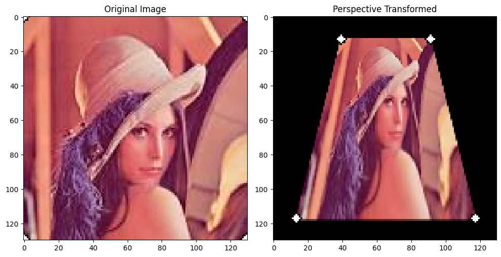

강도 변환 (Intensity Transformations)

강도 변환은 이미지의 픽셀 값 자체를 변환 하는 것입니다.

• 히스토그램 평활화, 매칭
• 감마 보정 등..

💻 라이브러리 및 이미지 호출

import cv2
import numpy as np
import matplotlib.pyplot as plt

# 이미지 불러오기
image = cv2.imread('lenna.jpg', cv2.IMREAD_GRAYSCALE)

💻 히스토그램 Plot

# 히스토그램 계산
hist = cv2.calcHist([image], [0], None, [256], [0,256])

plt.figure()
plt.title("Lenna Image Histogram")
plt.xlabel("Bins")
plt.ylabel("# of Pixels")
plt.plot(hist)
plt.xlim([0, 256])
plt.show()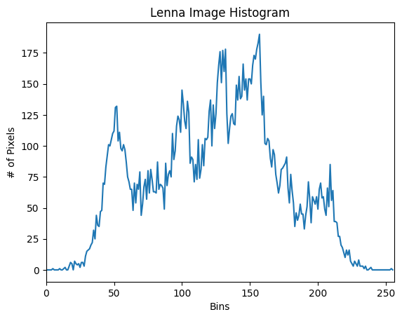

💻 히스토그램 평활화

# 이미지 불러오기
image = cv2.imread('lenna.jpg', cv2.IMREAD_GRAYSCALE)

# 히스토그램 평활화
equalized_image = cv2.equalizeHist(image)


fig, axes = plt.subplots(1, 2, figsize=(5, 10))
axes[0].imshow(image, cmap='gray')
axes[1].imshow(equalized_image, cmap='gray')
plt.show()

💻 히스토그램 매칭

def histogram_matching(source, reference):
    s_values, bin_idx, s_counts = np.unique(source, return_inverse=True, return_counts=True)
    r_values, r_counts = np.unique(reference, return_counts=True)

    s_quantiles = np.cumsum(s_counts).astype(np.float64)
    s_quantiles /= s_quantiles[-1]
    r_quantiles = np.cumsum(r_counts).astype(np.float64)
    r_quantiles /= r_quantiles[-1]

    interp_r_values = np.interp(s_quantiles, r_quantiles, r_values)
    matched = interp_r_values[bin_idx].reshape(source.shape)
    return matched

# 원본 이미지와 참조 이미지 불러오기
source = cv2.imread('lenna.jpg', cv2.IMREAD_GRAYSCALE)
reference = cv2.imread('ref.jpg', cv2.IMREAD_GRAYSCALE)

matched_image = histogram_matching(source, reference)

fig, axes = plt.subplots(2, 3, figsize=(15, 10))
# Images
axes[0, 0].imshow(source, cmap='gray')
axes[0, 0].set_title("Source Image")
axes[0, 1].imshow(reference, cmap='gray')
axes[0, 1].set_title("Reference Image")
axes[0, 2].imshow(matched_image, cmap='gray')
axes[0, 2].set_title("Matched Image")

# Histograms
axes[1, 0].hist(source.ravel(), 256, [0,256], color='black')
axes[1, 0].set_title("Source Histogram")
axes[1, 1].hist(reference.ravel(), 256, [0,256], color='black')
axes[1, 1].set_title("Reference Histogram")
axes[1, 2].hist(matched_image.ravel(), 256, [0,256], color='black')
axes[1, 2].set_title("Matched Histogram")

plt.tight_layout()
plt.show()

---