BinaryViT: Pushing Binary Vision Transformers Towards Convolutional Models

---

BinaryViT에 대한 내용

Abstract

Binarization은 weight와 activation이 binary 상태일 때, popcount 연산을 사용함으로써, ViT model의 크기와 computational cost를 크게 줄일 수 있다.

Vanilla ViT들은 CNN이 갖고 있는 핵심적인 구조적 특성들이 결여되어 있어, binary CNN보다 representational capability가 현저히 떨어진다.

1. Introduction

Activation, Weight 모두 binarize된 ViT의 accuracy를 full-precision model과 비슷하게 하기 위한 방법들

1. Distillation
2. Scaling factor를 learnable parameter로 설정
3. Bi-RealNet: 추가적인 residual connection을 통해, 정보를 보존
4. ReActNet: sign함수 앞에 learnable threshold를 추가하고, 각 residual connection 뒤에 RPReLU activation 함수를 추가하여, output distribution을 재구성
5. BiMLP: multibranch block을 제안하여 patch 혼합과, channel 혼합이 동시에 이루어지게 하여, FC layer의 제한된 표현력을 극복

2. Designing a full binarized ViT baseline

CNN과 BERT에 적용된 기존 binarization 기법을 활용하여, A1W1 Vanilla ViT 설계

2.1. Binarized fully-connected layer

$X∈{\R}^{N⨉D_{in} }$에 sign()를 적용하기 직전에,
threshold vector ${\beta}_X∈{\R}^{D_{in}}$를 적용한다.

$W∈{\R}^{D_{in}⨉D_{out}}$의 threshold는 ${\mu}(W)∈\R^D_{out}$이다. ${\mu}(W)$는 $W$의 평균이다.

전체 행렬 곱셈식은 다음과 같다.
$Y(X) = \alpha_Wsign(X+\beta_X) ⊗ sign(W-\mu(W))$

실제 구현은 조금 다르다($\beta_X$가 없고, popcount가 아니며, $\alpha_W$가 $Sign(W - \mu(W))$에 곱해진다. 아래 코드를 실행하면 그 과정을 알 수 있다.

PS) 아니다, $\beta_X$가 없는게 아니고, $Y(X)$를 호출하는 쪽에서 $X+\beta_X$처리를 하고, $X$로 넣기에 BinaryQuantizer에 없는 것이다.

import torch
import torch.nn as nn

# BinaryQuantizer: 이진 양자화를 위한 autograd.Function
class BinaryQuantizer(torch.autograd.Function):
    @staticmethod
    def forward(ctx, input):
        # forward 단계: 입력 텐서를 이진화 (부호 함수: -1, 0, 1 반환)

        ctx.save_for_backward(input)  # backward 단계에서 사용하기 위해 입력 저장
        out = torch.sign(input)
        return out

    @staticmethod
    def backward(ctx, grad_output):
        # backward 단계: 기울기를 계산함

        input = ctx.saved_tensors  # 저장한 입력값을 불러옴
        input = input[0]
        # 입력이 [-1, 0] 구간에 해당하는지 판별 (float 텐서로 변환)
        indicate_leftmid = ((input >= -1) & (input <= 0)).float()
        # 입력이 (0, 1] 구간에 해당하는지 판별
        indicate_rightmid = ((input > 0) & (input <= 1)).float()
        # 각 구간에 대해 선형 보정된 기울기를 계산한 후 grad_output과 곱함
        grad_input = (indicate_leftmid * (2 + 2 * input) + indicate_rightmid * (2 - 2 * input)) * grad_output.clone()
        return grad_input
    
    # QuantizeLinear: 양자화된 선형(fully-connected) 계층

class QuantizeLinear(nn.Linear):
    def __init__(self,  *kargs, bias=False, config=None):
        super(QuantizeLinear, self).__init__(*kargs, bias=bias)
        # 가중치와 입력의 양자화 비트 수를 config에서 가져옴
        self.weight_bits = config.weight_bits
        self.input_bits = config.input_bits
        
        # 가중치 양자화 방법 선택 (비트 수에 따라 다른 양자화 함수 사용)
        if self.weight_bits == 1:
            self.weight_quantizer = BinaryQuantizer
        elif self.weight_bits == 2:
            # self.weight_quantizer = TwnQuantizer
            # 가중치 클리핑 범위를 버퍼에 등록
            self.register_buffer('weight_clip_val', torch.tensor([-config.clip_val, config.clip_val]))
        elif self.weight_bits < 32:
            # self.weight_quantizer = SymQuantizer
            self.register_buffer('weight_clip_val', torch.tensor([-config.clip_val, config.clip_val]))
            
        # 입력(activation) 양자화 방법 선택
        if self.input_bits == 1:
            self.act_quantizer = BinaryQuantizer
        elif self.input_bits == 2:
            # self.act_quantizer = TwnQuantizer
            self.register_buffer('act_clip_val', torch.tensor([-config.clip_val, config.clip_val]))
        elif self.input_bits < 32:
            # self.act_quantizer = SymQuantizer
            self.register_buffer('act_clip_val', torch.tensor([-config.clip_val, config.clip_val]))
 

    def forward(self, input):
        
        # 가중치 양자화: 비트 수에 따라 다르게 처리
        if self.weight_bits == 1:
            print("=== Weight ===\n")
            print(f"W : {self.weight}\n")

            # 이진 가중치의 경우, 각 행별 평균 절댓값을 스케일링 팩터로 사용
            scaling_factor = torch.mean(abs(self.weight), dim=1, keepdim=True)
            print(f"a_W : {scaling_factor}\n")
            scaling_factor = scaling_factor.detach()

            real_weights = self.weight - torch.mean(self.weight, dim=-1, keepdim=True)
            print(f"M(W) : {torch.mean(self.weight, dim=-1, keepdim=True)}\n")
            print(f"W - M(W) : {real_weights}\n")

            binary_weights_no_grad = scaling_factor * torch.sign(real_weights)
            print(f"sign(W - M(W)) : {torch.sign(real_weights)}\n")

            cliped_weights = torch.clamp(real_weights, -1.0, 1.0)
            # 이진화된 가중치로 기울기 흐름은 유지하면서 클램핑된 값을 사용
            weight = binary_weights_no_grad.detach() - cliped_weights.detach() + cliped_weights
            print(f"a_W * sign(W - M(W)) : {weight}\n")
        elif self.weight_bits < 32:
            # 지정된 양자화 함수를 적용하여 가중치를 양자화
            weight = self.weight_quantizer.apply(self.weight, self.weight_clip_val, self.weight_bits, True)
        else:
            # 양자화를 사용하지 않는 경우 원래의 가중치를 사용
            weight = self.weight

        # 입력(activation) 양자화: 입력이 이진인 경우에만 적용
        if self.input_bits == 1:
            print("=== Activation ===\n")

            print(f"X : {input}\n")
            input = self.act_quantizer.apply(input)
            print(f"sign(X + b_X) : {input}\n")
                
        # 선형 연산 수행
        print("=== Y ===\n")
        out = nn.functional.linear(input, weight)
        print(f"(sign(X + b_X)) * (a_W * sign(W - M(W))) : {out}\n")

        # bias가 존재하면 bias 추가 (출력 텐서 크기에 맞게 확장)
        if not self.bias is None:
            out += self.bias.view(1, -1).expand_as(out) 

        return out
    
    
# ------------------------------------------------------------------------------
# 테스트 코드를 위한 DummyConfig 클래스 정의 (실제 config 대신 사용)
class DummyConfig:
    def __init__(self, weight_bits, input_bits, clip_val):
        self.weight_bits = weight_bits
        self.input_bits = input_bits
        self.clip_val = clip_val

# QuantizeLinear 테스트 함수
def test_quantize_linear():
    print("\n=== QuantizeLinear 테스트 ===\n")
    # Dummy config 생성: 가중치와 입력 모두 1비트, 클리핑 값 1.0
    config = DummyConfig(weight_bits=1, input_bits=1, clip_val=1.0)
    # 입력 차원 5, 출력 차원 3인 QuantizeLinear 계층 생성
    qlinear = QuantizeLinear(5, 3, bias=False, config=config)
    # print(f"초기 W : {qlinear.weight}\n")

    # 더미 입력 생성: 배치 크기 2, 입력 차원 5
    dummy_input = torch.randn(2, 5)
    # print(f"X : {dummy_input}\n")
    
    # forward pass 실행
    output = qlinear(dummy_input)
    print(f"Y : {output}\n")

if __name__ == "__main__":
    test_quantize_linear()

이렇게 행렬 곱셈 이후엔, Batch Normalization을 적용하고, residual connection을 연결하고, RPReLU activation function을 적용한다.

$BiFC(X) = RPReLU[BN\{\alpha_Wsign(X+\beta_X) ⊗ sign(W-\mu(W))\} + R(X)]$

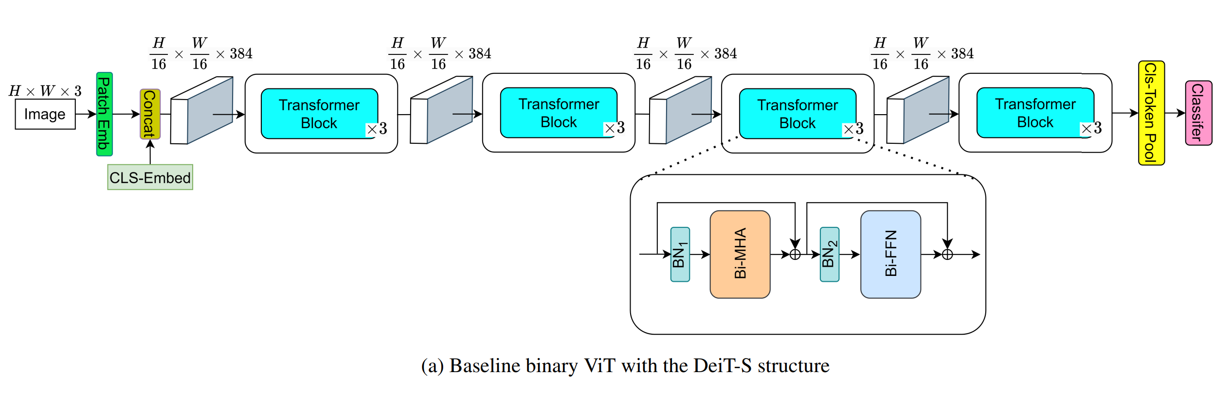
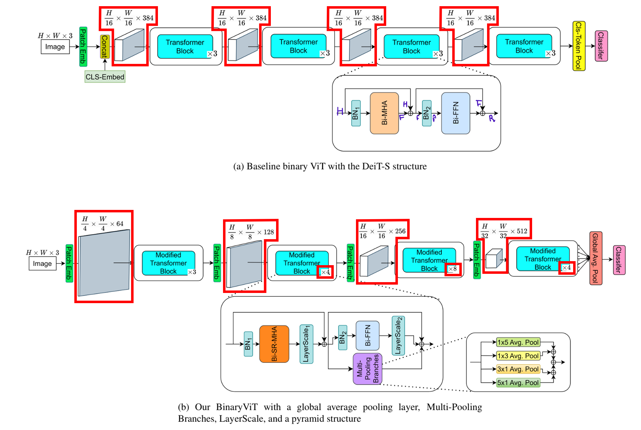
2.2. Binarized vision transformer

기존 Binary ViT의 과정

1. 처음 이미지 $x∈\R^{H⨉W⨉C}$는 embedding layer에서, patch $x_p∈\R^{N⨉(P^2•C)}$로 분할된다. (이때, patch의 수 $N = HW/P^2$이다.)
   
   

2. 각 patch에 대해 linear projection, $E∈\R^{(P^2⨉C)⨉D}$가 적용되어, $x∈\R^{N⨉D}$가 되고,
   class token embedding $x_{class}∈\R^D$가 추가되어 $x∈\R^{(N+1)⨉D}$가 되고,
   position embedding $E_{pos}∈\R^{(N+1)⨉D}$가 더해져,
   $H∈\R^{(N+1)⨉D}$가 출력된다.
   
   $H = [\mathbf{x}_{class}; \mathbf{x}_p^1E; \mathbf{x}_p^2E; ,,,; \mathbf{x}_p^NE] + E_{pos}$
   (';'는 행방향으로 붙이는 것임)
   
   

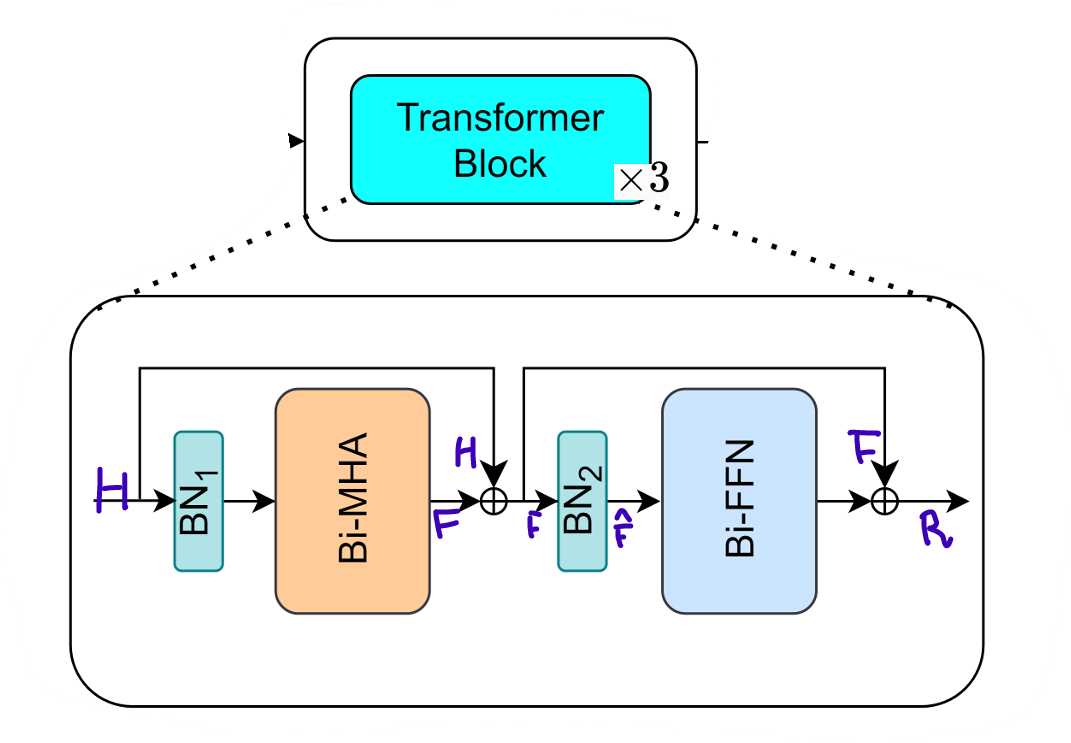
3. Embedding layer의 output $H∈\R^{(N+1)⨉D}$가 첫 번째, transformer block(encoder block)에 입력으로 들어간다.
   
   

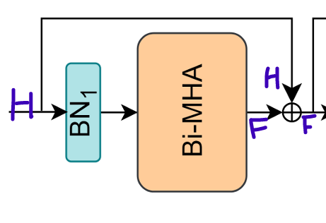
4. Transformer block에서 입력 $H∈\R^{(N+1)⨉D}$는 pre-batch-normalization layer를 거쳐, $\hat{H} = BN_1(H) ∈ \R^{(N+1)⨉D}$로 변환 된다.
   
   

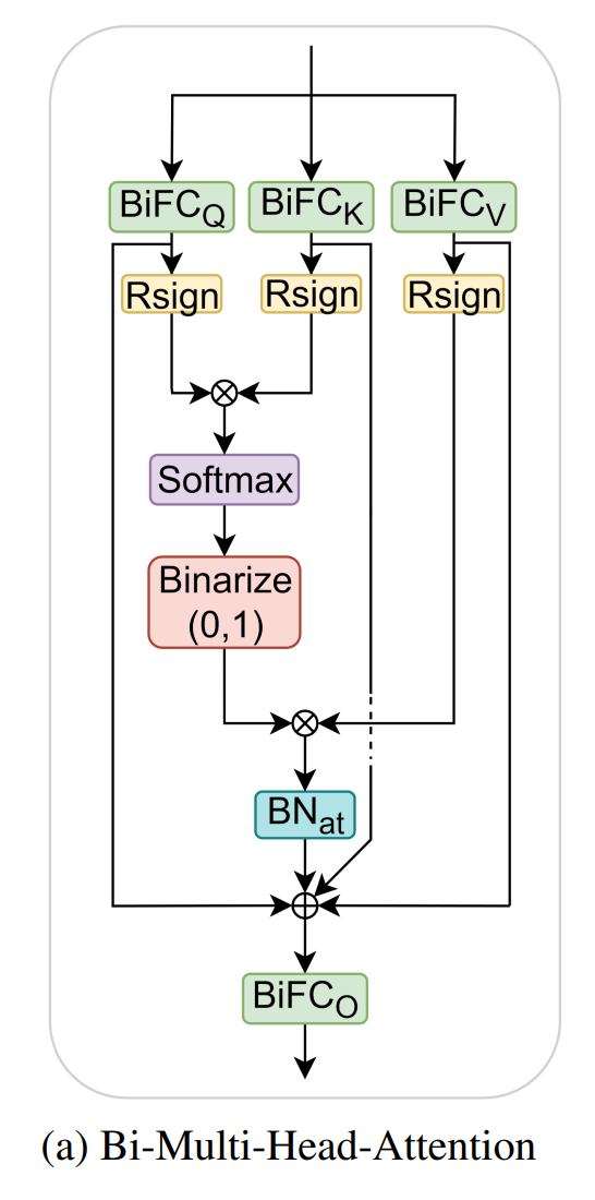
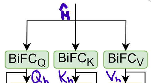
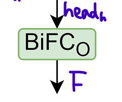
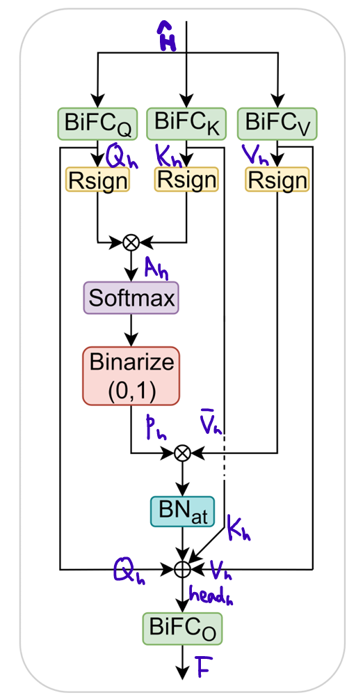
5. $N_H$개의 atttention head를 가진 binarized된 MHA module에서 $\hat{H}$를 BiFC(Binarized FC)에 넣으면, $Q_h,K_h,V_h$가 다음과 같이 계산된다.
   
   $Q_h=BiFC_{Q_h}(\hat{H}_h)∈\R^{(N+1)⨉D_h}$
   $K_h=BiFC_{K_h}(\hat{H}_h)∈\R^{(N+1)⨉D_h}$
   $V_h=BiFC_{V_h}(\hat{H}_h)∈\R^{(N+1)⨉D_h}$
   
   $D_h=D/N_H$
   
   

6. Attention score 구하기. Attention score은 다음과 같이 계산된다.
   $A_h=Rsign(Q_h)•Rsign(K_h^T)∈\R^{(N+1)⨉(N+1)}$
   
   

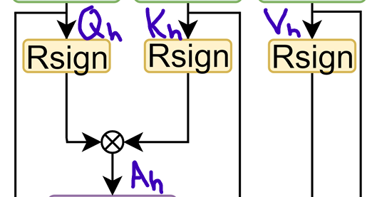
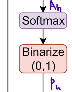
7. Attention score $A_h$를 softmax하고, 0 또는 1로 binarize하여, attention probability를 얻는다. 그 식은 다음과 같다.
   
   $\mathbf{P}_h = \alpha_{\mathbf{P}} \left[ \sigma \left( \frac{1}{\alpha_{\mathbf{P}}} \mathrm{Softmax} \left( \frac{\mathbf{A}_h}{\sqrt{D_h}} \right), 0, 1 \right) \right] ∈ \R^{(N+1)⨉(N+1)}$
   
   이때, $\alpha_P ∈ \R$는 learnable scaling factor이다.
   
   

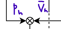
8. Attention probability $P_h ∈\R^{(N+1)⨉(N+1)}$를 $Rsign()$으로 binarized된 $\bar{V}_h=Rsign(V_h) ∈ R^{(N+1)⨉D}$과 곱하여, 각 token에 대해 value 정보를 반영한다.
   
   $P_h•\bar{V}_H∈ R^{(N+1)⨉D_h}$
   
   
   

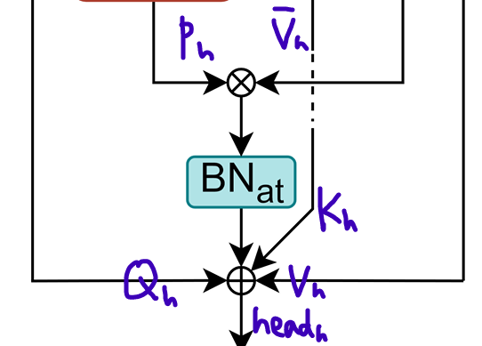
9. Token에 대한 value 정보가 반영된 attention probability를 BatchNormalization 해주고,
   Q, K, V 정보 보존을 위해, $Q_h, K_h, V_h$를 residual connection으로 연결한다.
   그 값을 RPReLU를 거치면, 하나의 head에 대한 output이 나온다.
   그 식은 아래와 같다.
   
   $head_h=RPReLU(BN_{at}(P_h\bar{V}_H)+Q_h+K_h+V_h)∈ \R^{(N+1)⨉D_h}$
   
   
   

10. 모든 head($N_H=D/D_h$)의 output($head_h$)는 서로 concatenate된 후, $BiFC$를 거치면, 전체 Bi-MHA의 output이 나온다.
    그 식은 아래와 같다.
    
    $F=BiFC_O(Cat(head_1, ..., head_{N_H}))∈ \R^{(N+1)⨉D}$
    
    
    

11. Main residual connection이 Bi-MHA의 output에 적용된다.
    그 식은 아래와 같다.
    
    $F=BiFC_O(Cat(head_1, ..., head_{N_H}))+H∈ \R^{(N+1)⨉D}$
    
    이때, $H$는 다음과 같고, 2번 과정에서의 $H$이다.
    
    $H = [\mathbf{x}_{class}; \mathbf{x}_p^1E; \mathbf{x}_p^2E; ,,,; \mathbf{x}_p^NE] + E_{pos}∈\R^{(N+1)⨉D}$
    
    
    

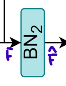
12. Residual output $F∈\R^{(N+1)⨉D}$는 두 번째 pre-batch-normalization layer인 $BN_2$를 거쳐 정규화된다.
    그 식은 아래와 같다.
    $\hat{F}=BN_2(F)∈\R^{(N+1)⨉D}$
    
    
    

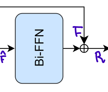
13. 정규화된 $\hat{F}∈\R^{(N+1)⨉D}$는 두 개의 BiFC로 구성된 BiFFN을 통과하고, 마지막으로 BiFFN의 output에 두 번째 main residual connection이 적용되어, 다음과 같이 최종 출력 $R$을 얻는다.
    $R=BiFFN(\hat{F})+F∈\R^{(N+1)⨉D}$
    
    
    

Distillation

Binarized된 ViT의 성능을 향상시키기 위해, student model의 logit과 teacher model의 logit 간의 soft crossentropy loss를 최소화함으로써, full-precision model의 knowledge를 binarized model로 distill한다.

3. What else do binary CNNs have that binary transformers do not have?

위 2장에서 언급된 모든 기법들을 적용하더라도 (Table 1의 ReActNet), 정확도가 낮다. 이는 대부분의 SOTA binary CNN 정확도보다 훨씬 낮다.
=> CNN architecture의 세부 요소 및 특성을 분석하여, ViT에 적용
=> Binary activation / weight로도 많은 수의 클래스를 가진 dataset에서도 accuracy ↑

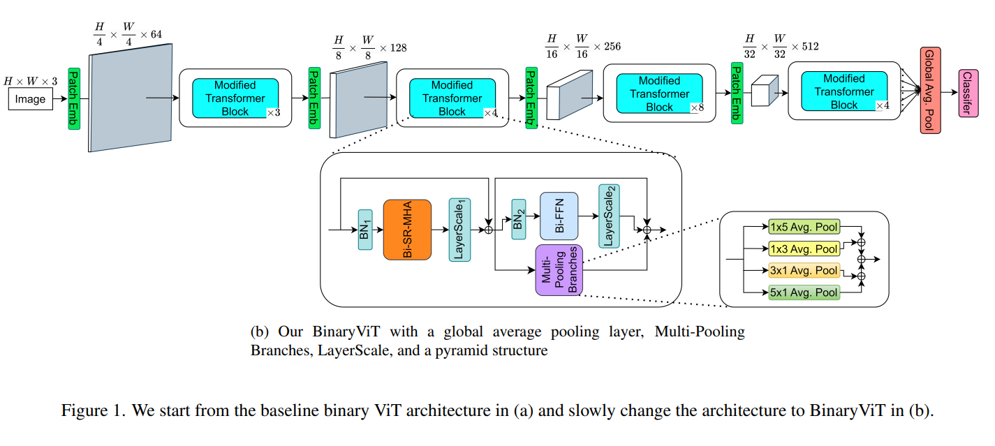
그러기 위해, Binary ViT의 표현력을 증가시키는 방법 3가지

1. Global Average Pooling(GAP)를 classifier layer 전에 삽입
   

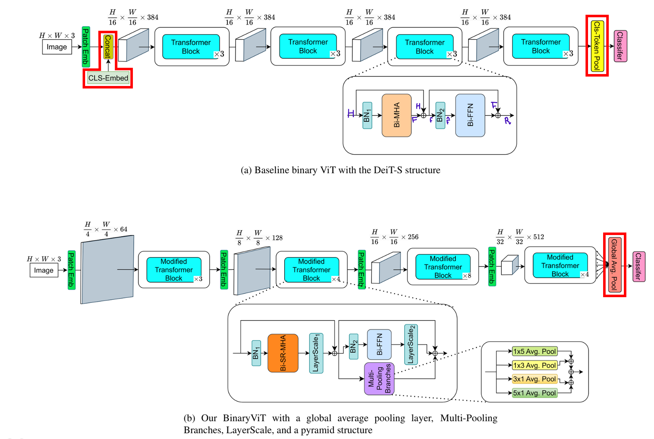
2. Multiple average pooling branch를 추가
   

3. CNN에서 피라미드 구조를 차용하기

추가적으로 ResNet, MobileNet의 설계 아이디어 차용

Main residual branch의 scale이 Bi-MHA, Bi-FFN 출력 같은 main branch의 scale을 압도하지 않도록 residual branch 앞에 affine 변환을 배치.

3.1. Global average pooling before classifier layer

Binary CNN: classifier 앞에 average pooling layer 有
Vanilla ViT: classifier 앞에 단일 cls-token pooling layer만 有

==> cls-token pooling을 Gloval average pooling(GAP)을 통해 모든 token 정보를 반영하자!
+
Embedding에서 cls-token embedding을 제거하자!

==> 위 2.2.의 과정 2의
$H = [\mathbf{x}_{class}; \mathbf{x}_p^1E; \mathbf{x}_p^2E; ,,,; \mathbf{x}_p^NE] + E_{pos}$ 이
$H = [\mathbf{x}_p^1E; \mathbf{x}_p^2E; ,,,; \mathbf{x}_p^NE] + E_{pos}$ 로 교체된다.
그렇게 되면 당연히, $H, E_{pos} ∈\R^{N⨉D}$ 가 된다.

// 연산량 소폭증가, 성능 대폭 증가

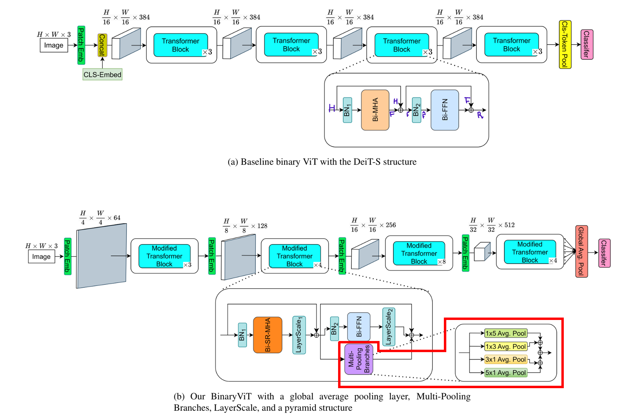
3.2. More branches

Binary Conv layer가 Binary FC layer보다 3배 정도 높은 표현력을 가진다.

==> Transformer block 내부의 Bi-FFN 옆에 4개의 average pooling branch를 추가.

각 average pooling layer는 다음과 같다.

• 1⨉5 Avg. Pool
• 1⨉3 Avg. Pool
• 5⨉1 Avg. Pool
• 3⨉1 Avg. Pool

// 연산량 소폭증가, 성능 대폭 증가

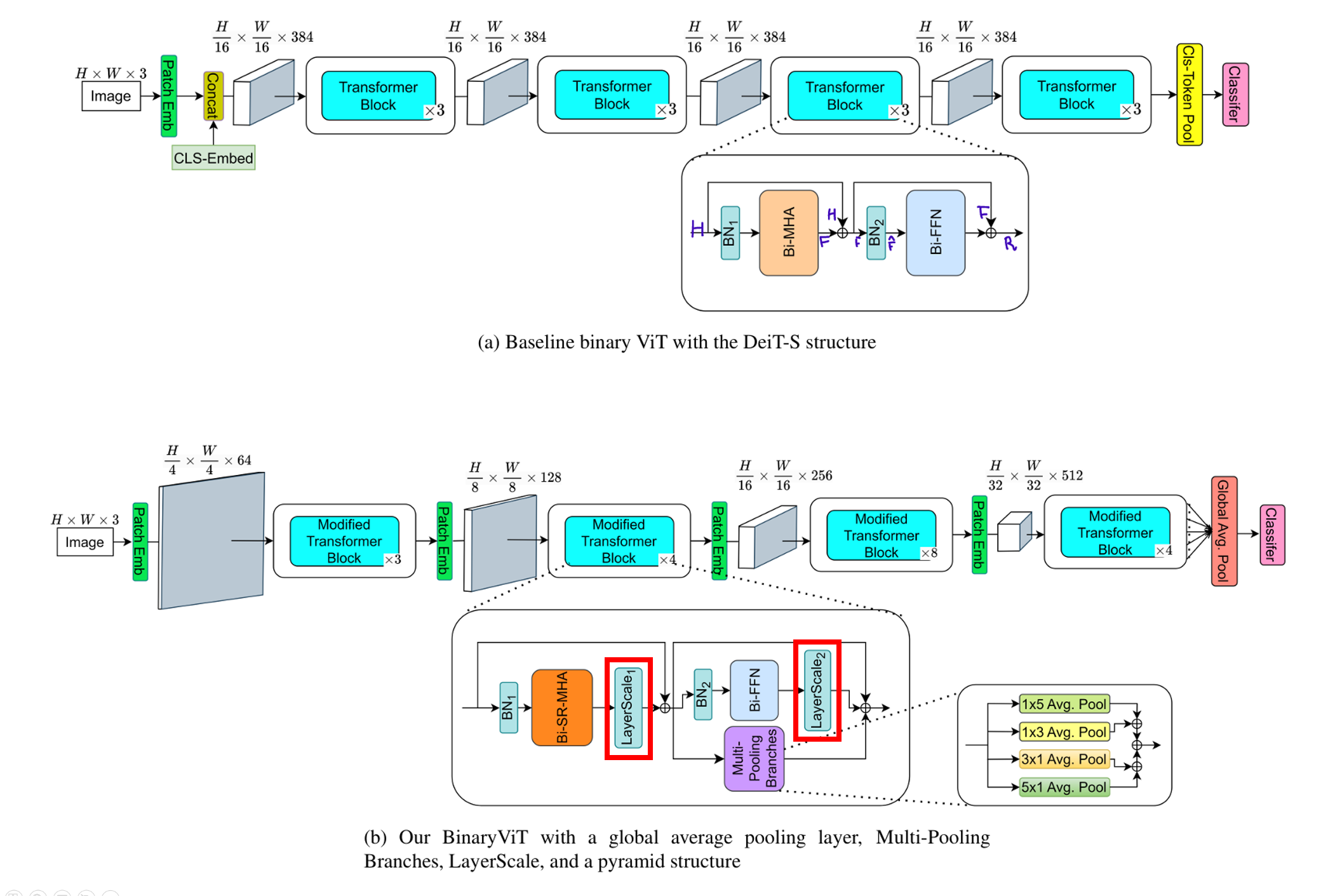
3.3. Scaling right before residual connection

사전 지식: Affine 변환(선형 변환으로 생각하면 됨)(ex, BN)은 model의 표현력에 영향을 미치지 않는다.

깊은 layer의 main branch에서 전달되는 정보가 residual branch에 의해 압도되어, 제 성능 발휘 못하는 문제가 생긴다.

Affine 변환이 표현력에 영향을 미치지 않지만,
여러가지 실험을 통해 residual connection 전에 affine 변환을 사용하는 것이 전혀 사용하지 않는 것보다 좋다는 것을 알게되었다.

==> Attention과 FFN의 각 main residual connection 마다 main branch(Bi-MHA, Bi-FFN의 output)에 affine 변환을 한다.

기존 방법

• $F=BiFC_O(Cat(head_1, ..., head_{N_H}))+H∈ \R^{(N+1)⨉D}$
• $R=BiFFN(\hat{F})+F∈\R^{(N+1)⨉D}$

Main branch에 Affine transformation 적용 방법

• $F=\alpha_1⊙BiFC_O(Cat(head_1, ..., head_{N_H}))+\beta_1+H∈ \R^{N⨉D}$
• $R=\alpha_2⊙BiFFN(\hat{F})+\beta_2+F∈ \R^{N⨉D}$
• $\alpha_1, \alpha_2, \beta_1, \beta_2 ∈ \R^{D}$

코드 비교

ReActNet

DATA_DIR=/path/to/dataset

torchrun --nproc_per_node=8 main.py \
    --num-workers=40 \
    --batch-size=64 \
    --epochs=300 \
    --dropout=0.0 \
    --drop-path=0.0 \
    --opt=adamw \
    --sched=cosine \
    --weight-decay=0.00 \
    --lr=5e-4 \
    --warmup-epochs=0 \
    --color-jitter=0.0 \
    --aa=noaug \
    --reprob=0.0 \
    --mixup=0.0 \
    --cutmix=0.0 \
    --data-path=${DATA_DIR} \
    --output-dir=logs/reactdeit-small-patch16-224 \
    --teacher-model-type=deit \
    --teacher-model=configs/deit-small-patch16-224 \
    --teacher-model-file=logs/deit-small-patch16-224/best.pth \
    --model=configs/deit-small-patch16-224 \
    --model-type=extra-res \
    --replace-ln-bn \
    --weight-bits=1 \
    --input-bits=1 \
    --enable-cls-token \
    --disable-layerscale \
    # --resume=logs/reactdeit-small-patch16-224/checkpoint.pth \
    # --current-best-model=logs/reactdeit-small-patch16-224/best.pth \

BinaryViT

DATA_DIR=/path/to/dataset

torchrun --nproc_per_node=8 main.py \
    --num-workers=32 \
    --batch-size=64 \
    --epochs=300 \
    --dropout=0.0 \
    --drop-path=0.0 \
    --opt=adamw \
    --sched=cosine \
    --weight-decay=0.00 \
    --lr=5e-4 \
    --warmup-epochs=0 \
    --color-jitter=0.0 \
    --aa=noaug \
    --reprob=0.0 \
    --mixup=0.0 \
    --cutmix=0.0 \
    --data-path=${DATA_DIR} \
    --output-dir=logs/binaryvit-small-patch4-224 \
    --teacher-model-type=deit \
    --teacher-model=configs/deit-small-patch16-224 \
    --teacher-model-file=logs/deit-small-patch16-224/best.pth \
    --model=configs/binaryvit-small-patch4-224 \
    --model-type=extra-res-pyramid \
    --replace-ln-bn \
    --weight-bits=1 \
    --input-bits=1 \
    --avg-res3 \
    --avg-res5 \
    # --resume=logs/binaryvit-small-patch4-224/checkpoint.pth \
    # --current-best-model=logs/binaryvit-small-patch4-224/best.pth \

ReActNet, BinaryViT 두 코드 모두에서의 Transformer block(class ViTLayer(nn.Module))에서Bi-MHA, Bi-FFN이 호출하는 class ViTOutput(nn.Module)

class ViTOutput(nn.Module):
    def __init__(self, config: ViTConfig, layer_num, drop_path=0.0) -> None:
        super().__init__()
        self.dense = QuantizeLinear(config.intermediate_size[config.stages[layer_num]], config.hidden_size[config.stages[layer_num]], config=config)
        self.dropout = nn.Dropout(config.hidden_dropout_prob)
        self.drop_path = DropPath(drop_path) if drop_path > 0. else nn.Identity()

        self.move = nn.Parameter(torch.zeros(config.intermediate_size[config.stages[layer_num]]))
        self.norm = config.norm_layer(config.hidden_size[config.stages[layer_num]], eps=config.layer_norm_eps)
        self.rprelu = RPReLU(config.hidden_size[config.stages[layer_num]])
        self.pooling = nn.AvgPool1d(config.intermediate_size[config.stages[layer_num]] // config.hidden_size[config.stages[layer_num]])
        self.layerscale = LayerScale(config.hidden_size[config.stages[layer_num]]) if not config.disable_layerscale else nn.Identity()


    def forward(self, hidden_states: torch.Tensor) -> torch.Tensor:
        out = self.norm(self.dense(hidden_states + self.move)) + self.pooling(hidden_states)
        out = self.rprelu(out)
        out = self.dropout(out)

        out = self.layerscale(out)

        out = self.drop_path(out)

        return out

위 2개의 script를 보면,
ReActNet의 방법에서는 --disable-layerscale을 통해, **Affine 변환을 disable하고 있어, self.layerscale = nn.Identity()로 아무 일이 일어나지 않다.

반면, BinayViT에서는 Affine 변환을 하고 있음을 알 수 있다.

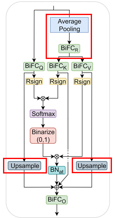
3.4. Pyramid structure

최신 SOTA Binary CNN은 고해상도에서 저해상도로 점진적으로 feature map 크기를 줄이고, hidden dimension은 증가시키는 pyramid structure를 갖는다.

이런 pyramid structure는 binary nn의 표현력을 향상시킨다.

==> pyramid structure를 통해, 계산 복잡도를 증가시키지 않으면서도, 표현력 ↑

첫 번째와 두 번째 스테이지에서 sequence size가 3316과 784이므로, 이 크기에서 attention을 적용하는 것은 계산 비효율적이다.

==> key, value 행렬을 계산하기 직전에 입력에 downsampling을 한다.

이렇게 downsampling된 값들은 residual connection 이전에 upsampling된다.

그 전체 식은 아래와 같다.

$head_h = RPReLU(BN_{at}(P_h\bar{V}_h) + Q_h + N(K_h) + N(V_h)$
여기서 $N()$은 upsampling으로, nearest-neighbor interpolation function이다.

$K_h=BiFC_{K_h}(BiFC_R(AvgPool(\hat{H}))_h)$
$V_h=BiFC_{V_h}(BiFC_R(AvgPool(\hat{H}))_h)$

$AvgPool()$은 kernel 크기와 stride가 R인 average pooling이다.

• 피라미드 코드의 ViTEncoder 부분의 ViTLayer를 반복 호출하는 루프에서 PatchEmbed 클래스를 주기적으로 호출하는 부분이다.