Mixed-Precision Neural Network Quantization via Learned Layer-wise Importance

---

MPQ via Learned Layer-wise Importance에 대한 내용

Abstract.

Scale factor를 특정 bit-width에서 최종 accuracy에 대한 해당 layer의 기여도를 반영하는 importance indicator로 사용.

Scale factor는 QAT 중에 수치적 변환을 자연스럽게 인지해서, 해당 layer의 quatization sensitivity indicator로서 효과적.

Joint training scheme을 통해 다양한 bit-width에 대한 지표를 한 번에 얻을 수 있음.

1 Introduction

Uniform-precision Q는 suboptimal임
⇒ Mixed-precision Q

MPQ에서 bit-width를 더 finer-grained
⇒ search space가 exponentially ↑

layer 수: $L$,
한 layer에서 activation에 대해 선택 가능한 bit-widht: $n$,
한 layer에서 weight에 대해 선택 가능한 bit-widht: $n$,
⇒ search scape $= L ⨉ (n+n)$

search-based MPQ

HAQ[25], AutoQ[21]:
bit-width 결정 문제를 Markov Decision Process로 modeling해서 Deep Reinforced Learing 활용.
⇒ 시간 ↑

DNAS[26], SPOS[14]:
differentiable search process를 달성하기 위해, NAS algorithm을 적용.
⇒ search space를 수동으로 제한

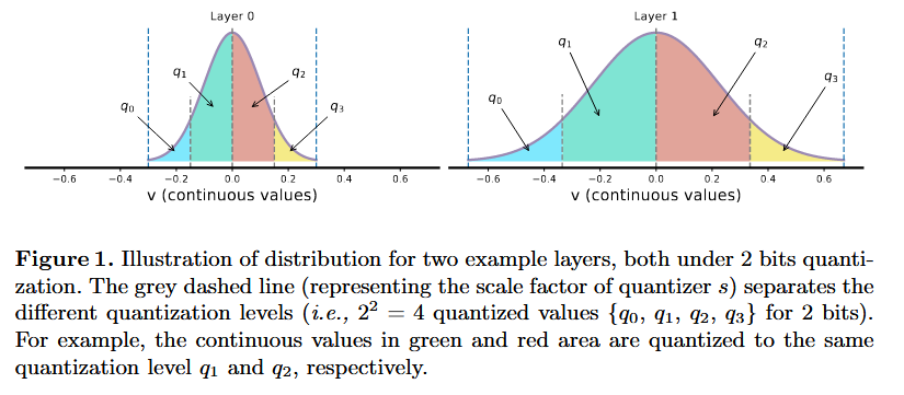
criterion-base MPQ

HAWQ[12], HAWQ-v2[11]:
layer의 sensitivity를 측정하기 위해, 2차 정보(hessian eigenvalue, trace)를 사용.
MPQCO[6]:
Hessian matrix를 효율적으로 계산 후, MCKP를 공식화.
⇒ Biased approximation:
Q되지 않은 network의 hessian 정보를 사용 ⇒ Q의 존재 인지 X
⇒ Limited search space:
MPQCO의 근원적인 문제로 인해...

⇒ End-to-end importance criterion 사용!
⇒ Q에 있는 learnable scale factor를 사용!

Scale factor는 end-to-end로 학습되므로,
Biased approximation X + limited search space X

+ joint training scheme을 통해, cirterion을 얻는 시간 ↓

2 Related Work

2.1 Neural Network Quantization

Fixed-Precision Quantization

• Lq-nets[28]: learnable quantizer 도입
• Pact [7]: activation을 위한 learnable upper bound 도입
• D.S. Learned step size quantization[13], Learning to quantize deep networks by optimizing quantization intervals with task loss.[18]: learnable scale factor 도입

Mixed-Precision Quantization

위에서 충분히 언급함

2.2 Indicator-Based Model Compression

위에서 충분히 언급함

3 Method

3.1 Quantization Preliminary

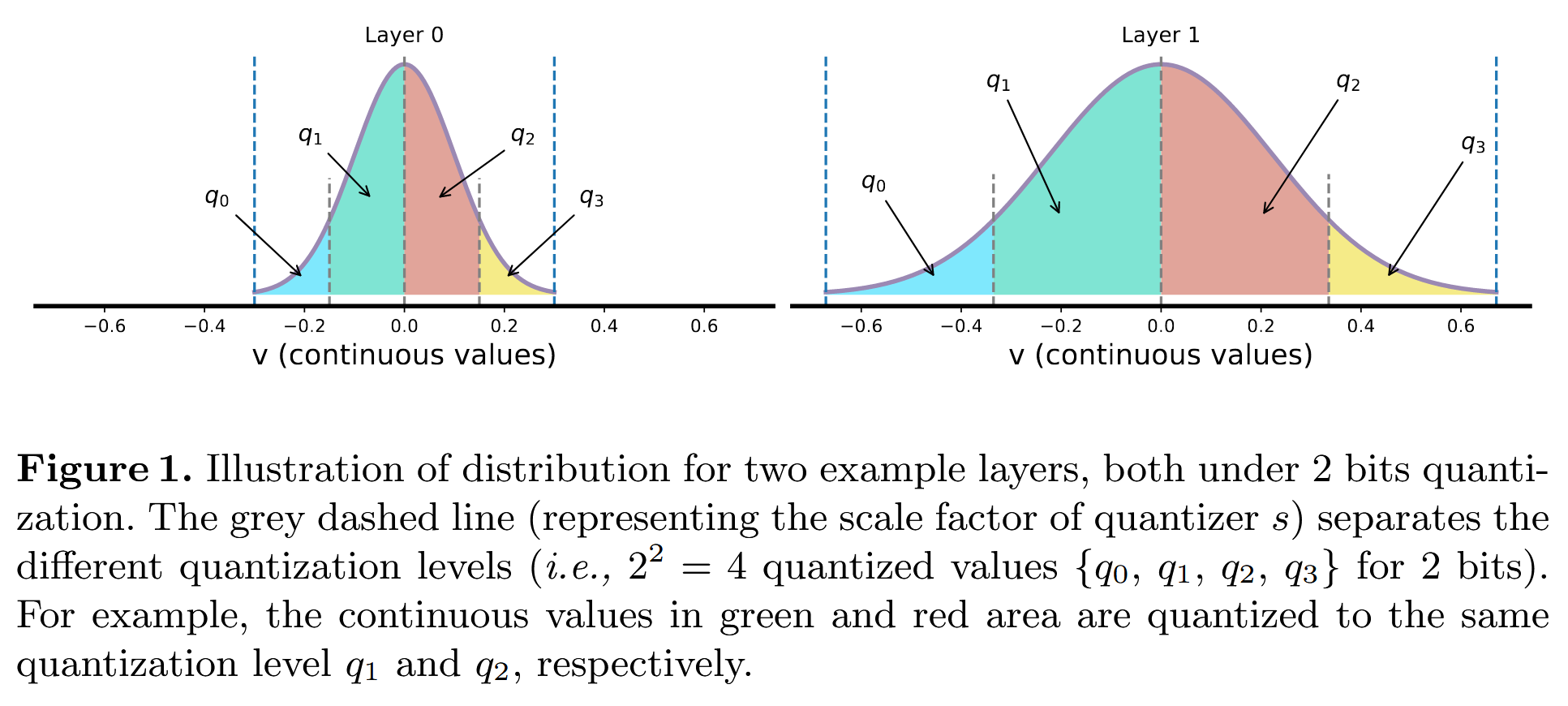
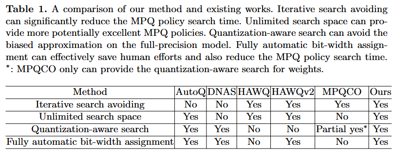
Scale factor ↑ ⇒ 더 많은 서로 다른 연속적인 값들이 동일한 Q된 값으로 mapping 됨

즉, Scale factor는 mapping 범위임

아래 그림 보면 Layer 1이 더 넓은 연속적인 수를 하나로 뭉뚱그림

3.2 From Accuracy to Layer-wise Importance

위 3a, 3b 제약 조건 下 $S^*$를 찾아함.

식의 의미:
$S$: 전체 network의 구성 bit-width임. (e.g., $L_1 = (3bit, 2bit), L_1 = (5bit, 6bit) ...$)

즉, 특정 Q 정책 $S$를 써서, train한 loss의 최소값을 갖는 parameter $W$를 $W_S$로 하고 (3a),
특정 $BitOps(S) ≤ C$를 지키면서,

valid ACC가 최대화 되는 S를 제한된 search space $\Gamma(\mathcal{A})$에서 찾겠다의 의미!!!

근데 search space $\mathcal(A)$가 너무 크니까 시간 오래걸리니까

⇒ joint training scheme

3.3 Learned Layer-wise Importance Indicators

같은 bit-width로 잘 훈련된 $s$와 weight를 가진 2개의 예시 layer를 Q해 봤을 때,

그림 1에서 볼 수 있듯이, layer 1의 분포가 layer 0보다 훨씬 넓다.

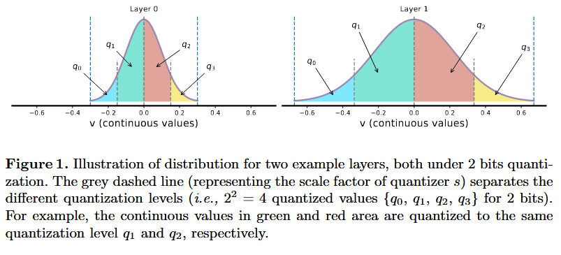
layer 1에서는 더 많은 서로 다른 연속적인 값들이 동일한 Q된 값으로 mapping
⇒ $s$ ↑
⇒ 원래 연속적인 값들의 내재된 차이를 더 많이 소멸 시켜 expressiveness ↓
⇒ bit-width 늘려야 함

$s$ ↑ ⇒ 중요함 ⇒ bit-width ↑

Feasibility Verification

MobileNet에서
Q sensitivity: depth-wise conv > point-wise conv
라고 알려짐.

MobileNetv1에 있는 5개의 DW-PW 쌍 각각에 대해, 개별적으로 Q해가며, scale factor와 accuracy를 측정.

총 10개의 실험을 함.

DW-PW 0을 2, 4 bit Q,
DW-PW 1을 2, 4 bit Q,
DW-PW 2를 2, 4 bit Q,
DW-PW 3을 2, 4 bit Q,
DW-PW 4를 2, 4 bit Q.

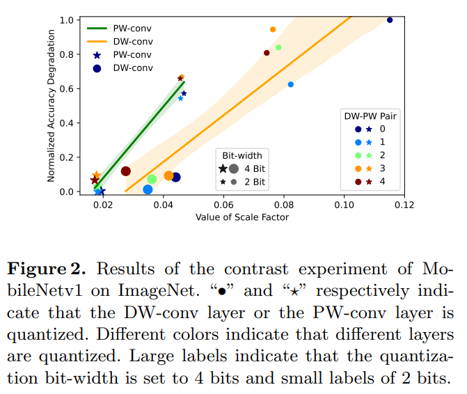
그림 2를 보면,

• 4bit에서 2bit로 감소할 때, DW-convs의 accuracy degradation이 더 큼
  ⇒ DW-convs가 매우 민감하다는 사전 지식과 일치
• 동일 bit-width에서 DW-convs의 scale factor가 더 큼
  ⇒ scale factor가 해당 layer의 Q sensitivity를 반영함

3.4 One-time Training for Importance Derivation

중요도 지표를 뽑는 cost ↑

⇒ 한 번의 훈련으로 모든 layer의 n개 bit-width에 해당하는 중요도 지표를 얻기 위한 joint training scheme

각 훈련 step $t$에서,
n개의 bit-width 옵션들에 대해, forward, backward를 n번 수행,
+ one-shot NAS에서 영감을 받아, 각 layer에 대해 무작위 bit-width 할당 과정을 한 번 도입하여, 다른 layer의 서로 다른 bit-width들이 서로 소통할 수 있게 함.

⇒ 한 step에서, gradient 계산 $n+1$번 수행.

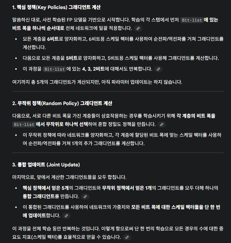
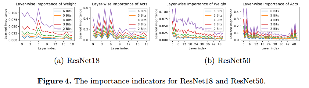
그림 4는 이 방법으로 단일 훈련 세션(물론 gradient 계산 $n+1$번)에서 얻은 모든 layer의 importance indicator를 나타냄.

3.5 Mixed-Precision Quantization Search Through Layer-wise Importance

그림 2에서 보았듯이, DW-convs가 높은 중요도 점수를 갖음
⇒ bit-width ↑

제약사항을 지키면서, 각 bit-width 별 중요도 점수의 총합이 가장 작은 조합을 찾으면 됨!

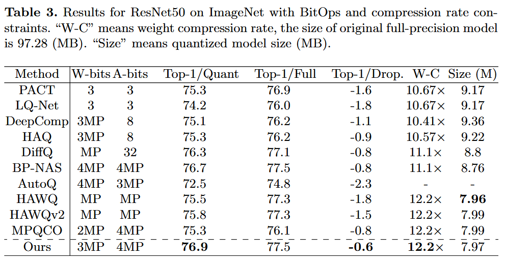
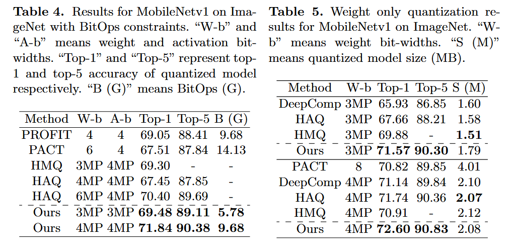
4 Experiments

Dataset: ImageNet
Model: ResNet18, ResNet50, MobileNetv1

• UniQ Baseline들: PACT[7] (PACT), PROFIT[23], LQ-Net[28]
• MixQ Baseline들: HAQ [25], AutoQ [21], SPOS [14], DNAS [26], BP-NAS [27], MPDNN [24], HAWQ [12], HAWQv2 [11], DiffQ [9], MPQCO [6]

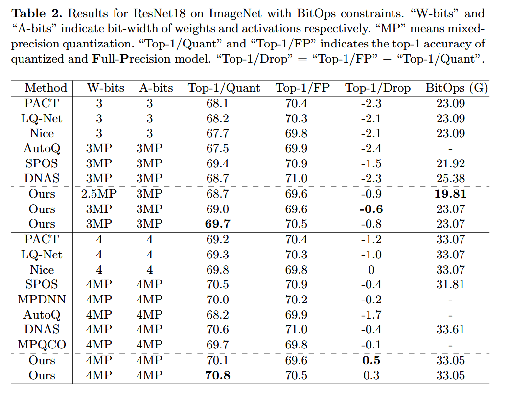
4.1 Mixed-Precision Quantization Performance Effectiveness

4.2 Mixed-Precision Quantization Policy Search Efficiency

4.3 Ablation Study

생략

5 Conclusion

생략