SmoothQuant: Accurate and Efficient Post-Training Quantization for Large Language Models

---

SmoothQuant에 대한 내용

Abstract

LLM inference Quantization for accuracy + hardware efficiency
==> SmoothQuant

SmoothQuant의 3가지 목표

1. training-free
2. accuracy-preserving
3. general-purpose PTQ

위 목표는 8-bit weight, 8-bit activation (W8A8) quantization으로 이룰 수 있다.

SmoothQuant는 weight quant가 activation quant 보다 쉽다는 점에 기반하여, activation의 outlier(극단값)을 부드럽게 완화하여 quantization의 어려움을 activation에서 weight로 이전하는 수학적으로 동등한 변환을 수행

Q1. 왜 weight quantization이 activation quantization 보다 쉬운가?

A1.
Weight Quantization은 학습된 파라미터(Weight)에만 적용되므로, 추가적으로 입력 데이터에 따른 동적인 변화에 신경 쓰지 않아도 된다.
반면
Activation Quantization은 입력 데이터와 모델의 동작에 따라 결과값이 달라질 수 있으므로, 훈련 데이터 분포를 잘 반영하지 못하면 성능 저하가 심각할 수 있기 때문에.
+
Activation의 경우 outlier가 있음
weight의 분포는 비교적 uniform하고 flat하여, quantizing이 용이
반면
activation의 distribution은 outlier로 인해 ununiform하고, unflat해서, quantization 어려움

==> 여러 LLM model에서의 모든 matrix multiplication에 대해 weight, activation을 INT8로 quantization

---

1. Introduction

Q2. GPT-3 model은 1750억 개의 parameters를 가진다. 이때 parameter는 무엇인가? 또한 만약 FP16이면 저장 및 실행하려면 최소 몇 Byte의 메모리가 필요한가?

A2.
parameter는 matrix, bias에 들어있는 하나의 값의 총 개수를 의미한다.
16bit * 1750억
= 2조8000억 bit
= 350GB

LLM은 크기가 크다
==> computation 비쌈
==> quantization으로 LLM cost 줄이자

이때, weight, activation을 INT8로 Quantized하자.
==>
GPU 메모리 사용량 절반
+
matrix multiplication throughput 2배

SmoothQuant

LLM에 대해 정확하고, 효율적인 PTQ 솔루션임.

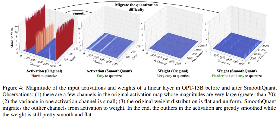
activation은 outlier로 인해 weight보다 quantization이 훨씬 어렵지만, 서로 다른 token은 channel간 유사한 변동성을 나타낸다.
==> SmoothQuant는 quantization의 어려움을 activation에서 weight로 이전하는 offline migration을 한다.

위 Figure 2에서 왼쪽 스케일을 잘 봐라. (a)의 경우 |X| (activation)는 0 ~ 10까지 큰 폭을 가져(outlier), quantizing하기 어렵다. 반면, (b)의 경우 그 어려움을 |Ŵ| (weight)로 offline migration하여, quantization을 쉽게 할 수 있게 하였다.

즉, SmoothQuant는 channel별로 수학적으로 동등한 스케일 변환을 제안하여 channel 간 크기를 크게 평탄화(smooth)하여 model을 quantization에 적합하게 한다.

---

2. Preliminaries

Integer Uniform Quantization

$\overline{X}^{INT8} = ⌊\frac{X^{FP16}}{Δ}⌉ , Δ = \frac{max(|X|)}{2^{N-1}-1}$ (1)

• $X$는 FP tensor
• $\overline{X}$는 quantization된 tensor
• $Δ$는 quantization step size (scaling factor)
• $⌊⋅⌉$는 반올림 연산
• $N$은 bit 수 (이 경우 8)

만약, tensor가 asymmetric이라면(ex) ReLU 이후) zero-point를 추가하여 처리할 수 있다.

이러한 quantization 방식은 activation의 outlier를 보존하기 위해 $max(|X|)$를 사용한다. (for accuracy 유지)

또한 $Δ$는 activation의 일부 calibraion sample을 사용하여 offline으로 계산할 수 있다. 이를 static quantization이라고 한다.

quantization granularity levels

• per-tensor quantization
  위 그림의 (a)이다. 이는 전체 matrix에 대해 single step size를 사용한다.
• per-token + per-channel quantization
  위 그림의 (b)이다. 이는 각 토큰에 연관된 activation에 대해 서로 다른 quantization step size를 사용하는 per-token quantization이나, weight의 각 output channel에 대해 다른 quantization step size를 사용하는 per-channel quantization를 적용할 수 있다.
• group-wise quantization
  이는 channel의 group 별로 서로 다른 quantization step size를 사용하는 방법이다.
  

---

3. Review of Quantization Difficulty

LLM에서 activation의 quantization이 어려운 이유
= outlier로 인해

1. Activations are harder to quantize than weights.

weight의 분포는 비교적 uniform하고 flat하여, quantizing이 용이
반면
activation의 distribution은 outlier로 인해 ununiform하고, unflat해서, quantization 어려움

2. Outliers make activation quantization difficult.

activation에서 나타나는 outlier의 크기는 대부분의 activation 보다 약 100배 이상 크다.
==>
per-tensor quantization에서
얼마 안되는 outlier 값들로 인해

$\overline{X}^{INT8} = ⌊\frac{X^{FP16}}{Δ}⌉ , Δ = \frac{max(|X|)}{2^{N-1}-1}$
에서 $max(|X|)$의 값이 너무 의미없이 커지게 된다.

즉, 얼마 안되는 outlier가 $Δ$를 지배하게된다.
==> non-outlier channel들이 무의미해 진다.

3. Outliers persist in fixed channels.

1. 한 channel에서 outlier가 발생하면, 특정 token에서만 outlier가 발생하는 것이 아닌, 모든 token에서 지속적으로 나타난다. (figure 4 참고)

2. channel 간 분산은 크고 (즉, 특정 token에 대해 일부 channel은 activation이 매우 크고, 나머지 channel은 작음. 즉, channel들 간 activation 크기 차이가 큼),
   channel 내 분산은 작다 (즉, 특정 channel에서의 activation은 여러 token 간 거의 일정하게 유지됨).

위 2가지 이유(outlier의 지속성, 각 channel 內의 작은 분산)로 인해, activation의 per-channel quantization을 수행할 수 있다면, per-tensor quantization과 비교했을 때 quantization error를 훨씬 줄일 수 있다. 이는 아래 Table 1에서 확인할 수 있다.

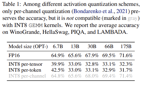
But,

per-channel quant는 hardware-accelerated GEMM kernel과 잘 맞지 않는다. 이 kernel은 높은 throughput을 요구하는 연산 sequence에 의존하며, 낮은 throughput을 가지는 instruction을 해당 sequence에 삽입하는 것을 허용하지 않는다.

==

==>

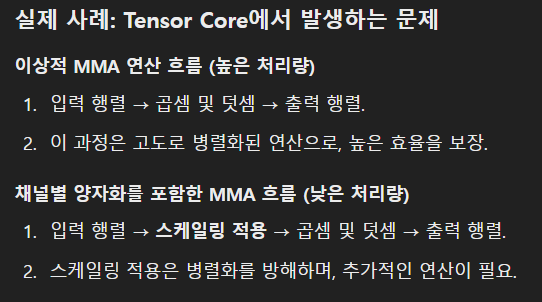
이전 연구들은 모두 linear layer에서의 per-token activation quantization을 사용하였으나, 이는 activation quantization의 어려움을 완전히 해결하지는 못함

---

4. SmoothQuant

위의 이유로인해 per-channel activation quantization 대신 acrivation을 smoothing factor $s ∈ R^{C_i}$로 나누어 smooth하고자 한다.

$Y = (X \cdot diag(s)^{-1}) \cdot (diag(s) \cdot W) =\hat{X} \cdot \hat{W}$ $(식 3)$

입력 $X$는 일반적으로 이전 linear operation으로 생성되므로, $s$는 이전 layer의 parameter에 offline으로 쉽게 병합할 수 있다.

==> 추가 scaling으로 인한 kernel overhead X

Migrate the quantization difficulty from activations to weights.

이 논문의 목표는 quantization의 어려움을 activation에서 weight로 이전 하는 것이다.

이를 위해 $s$를 선택하여 $\hat{X} = X \cdot diag(s)^{-1}$으로 quantization하기 쉬운 형태가 되도록 하고자 한다.

quantization error를 줄이기 위해, 모든 channel에서 effective quantization bits를 증가시켜야 하는데, effective quantization bits의 총합은 모든 channel이 동일한 최대 크기를 가질 때 가장 커진다.

// effective quantization bits : quantization 시 표현 가능한 데이터의 정확도.

==> 걍 outlier를 줄이려는 거임

==> $s_j = max(|X_j|), j=1,2,...,C_i$
예를들어,

의 $s$는 아래와 같다.

activation의 범위는 dynamic하다. 입력 sample에 따라 달라질 수 있다. 이를 해결하기 위해, pre-training dataset에서 calivration sample을 사용하여 activation channel의 scale을 추정한다.

But

모든 quantization 어려움이 weight로 이전된다.
==> weight quantization error ↑

∴ 반대로 $s_j = 1/max(|W_j|)$를 선택하면, quantization 어려움을 activation으로 이전한다.

==> 적절하게 합쳐야한다

==>
$\LARGE s_j = \frac{\max(|X_j|)^\alpha}{\max(|W_j|)^{1-\alpha}}$
$식(5)$

대부분의 model에서 $α = 0.5$일 때, quantization 어려움을 균등하게 분할함.

==> 해당 channel에서 weight와 activation이 유사한 최대 값을 가지도록 보장하여, 비슷한 quantization 어려움을 공유하게 한다.

// activation outlier가 더 두드러지는 model의 경우 $α = 0.75$가 더 낫다.

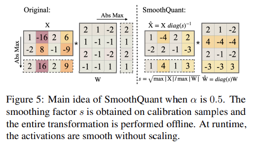
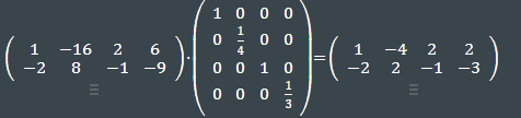
위 Figure 5는 $α = 0.5$일 때의 예시이다.

이때, $\hat{X} = X \cdot diag(s)^{-1}$은 다음과 같다.

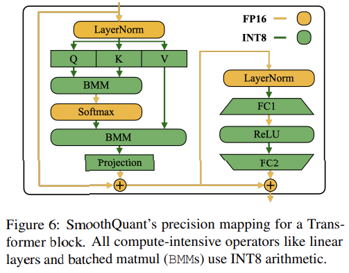
Applying SmoothQuant to Transformer block

LLM model에서 linear layer는 대부분의 parameter와 computation을 차지한다.

==> self-attention 및 feed-forward layer의 input activation에 대해 scale smoothing을 수행하고, 모든 linear layer를 W8A8로 quantization한다.
또한 attention 계산에서 BMM operator도 quantization 한다.

---

5. Experiments

생략

---

6. Related Work

생략

---

Conclusion

생략

---