머신러닝 - 차원축소

PCA

[PCA Parameters]

Packge : https://scikit-learn.org/stable/modules/generated/sklearn.decomposition.PCA.html
ncomponents : 몇개의 축으로 차원을 축소할 것인가
explained_variance : The amount of variance explained by each of the selected components.
explainedvariance_ratio : Percentage of variance explained by each of the selected components.

# PCA Fitting
pca = PCA(n_components = 20)
X_pca = pca.fit_transform(X)
print("PCA Output shape : {}".format(X_pca.shape))

PCA Output shape : (10000, 20)

def scree_plot(pca):
    num_components = len(pca.explained_variance_ratio_)
    ind = np.arange(num_components)
    vals = pca.explained_variance_ratio_
 
    plt.figure(figsize=(10, 6))
    ax = plt.subplot(111)
    cumvals = np.cumsum(vals)
    ax.bar(ind, vals)
    ax.plot(ind, cumvals)
    for i in range(num_components):
        ax.annotate(r"%s%%" % ((str(round(vals[i]*100,1))[:3])), (ind[i]+0.2, vals[i]), 
                    va="bottom", 
                    ha="center", 
                    fontsize=8)
 
    ax.xaxis.set_tick_params(width=0)
    ax.yaxis.set_tick_params(width=1, length=6)
 
    ax.set_xlabel("Principal Component")
    ax.set_ylabel("Variance Explained (%)")
    plt.title('Explained Variance Per Principal Component')
scree_plot(pca)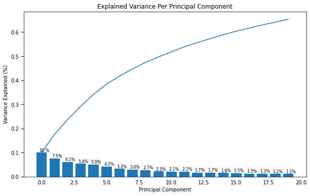

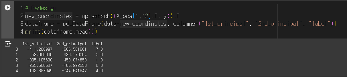
# Plotting
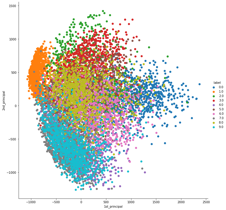
sns.FacetGrid(dataframe, hue="label", size=10).map(plt.scatter, '1st_principal', '2nd_principal').add_legend()
plt.show()

T-SNE

Packge : https://scikit-learn.org/stable/modules/generated/sklearn.manifold.TSNE.html
n_components : 몇개의 축으로 차원을 축소할 것 인가
perplexity : i 기준 주변 j를 몇개까지 고려할 것 인가
The perplexity is related to the number of nearest neighbors that is used in other manifold learning algorithms
Consider selecting a value between 5 and 50
default = 30
learning_rate : KL-Divergence를 최적화 할때 Gradient Descent를 활용함
GD를 할때 Learning rate 의미
The learning rate for t-SNE is usually in the range [10.0, 1000.0]
default='auto'
n_iter : GD iteration
Maximum number of iterations for the optimization
적어도 250번 이상 해야함
default = 1000
init : 처음 저차원에 대한 정보를 시작할때 기준점
{'random', 'pca'}
KL-Divergence 최적화 전 저차원의 분포와 고차원 분포를 setting 할때 사용
Initialization of embedding. PCA initialization cannot be used with precomputed distances and is usually more globally stable than random initialization.
default = 'pca'
method : Gradient 계산할 때 쓰는 알고리즘
{‘barnes_hut’, ‘exact’}
Barnes-Hut approximation : O(NlogN) time
exact : O(N^2) time
exact는 시간 많이 걸림
실험상 exact가 3% 더 에러가 적음
data가 작을 때는 exact로 돌리면 좋음
default=’barnes_hut’

%%time
# 2차원 t-SNE 임베딩 using barnes_hut
X_tsne_b = TSNE(n_components = 2, method='barnes_hut').fit_transform(X)

CPU times: user 2min 51s, sys: 500 ms, total: 2min 52s
Wall time: 1min 44s

# Redesign
new_coordinates_b = np.vstack((X_tsne_b[:,:2].T, y)).T
dataframe_b = pd.DataFrame(data=new_coordinates_b, columns=("Axis 1", "Axis 2", "label"))
# Plotting
sns.FacetGrid(dataframe_b, hue="label", height=10).map(plt.scatter, "Axis 1", "Axis 2").add_legend()
plt.show()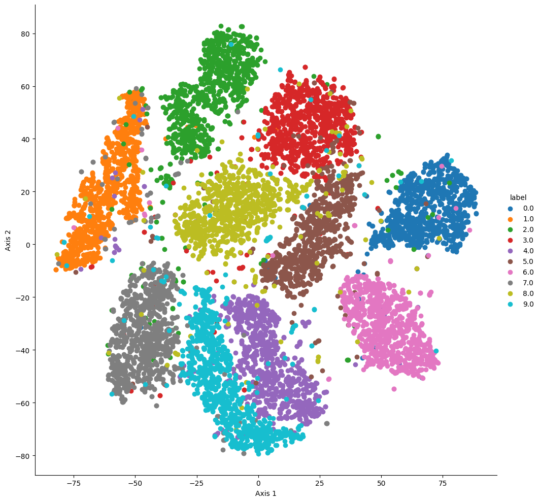

AutoEncoder

[Autoencoder Dense Parameters]

Packge : https://www.tensorflow.org/api_docs/python/tf/keras/layers/Dense
activation fuction : sigmoid가 기본이지만 Depth가 깊어질 수록 Gradient 문제가 발생하기 때문에 여러가지 function 들이 사용 됨
relu function
sigmoid function
softmax function
softplus function
softsign function
tanh function
selu function
elu function
exponential function
PReLU function
LeakyReLU function

# This is the dimension of the latent space (encoding space)
latent_dim = 2

# Images are 28 by 28
img_shape = (x_train.shape[1], x_train.shape[2])

encoder = Sequential([
    Flatten(input_shape=img_shape),
    Dense(192, activation='relu'),
    Dense(64, activation='relu'),
    Dense(32, activation='relu'),
    Dense(latent_dim, name='encoder_output')])

decoder = Sequential([
    Dense(64, activation='relu', input_shape=(latent_dim,)),
    Dense(128, activation='relu'),
    Dense(img_shape[0] * img_shape[1], activation='relu'),
    Reshape(img_shape)])

# iteration(epoch)에 따른 latent 1, 2의 변화
class TestEncoder(tf.keras.callbacks.Callback):
    def __init__(self, x_test, y_test):
        super(TestEncoder, self).__init__()
        self.x_test = x_test
        self.y_test = y_test
        self.current_epoch = 0

    def on_epoch_begin(self, epoch, logs={}):
        self.current_epoch = self.current_epoch + 1
        encoder_model = Model(inputs=self.model.input,
                              outputs=self.model.get_layer('encoder_output').output)
        encoder_output = encoder_model(self.x_test)
        plt.subplot(10, 5, self.current_epoch)
        plt.title("epoch : {}".format(self.current_epoch))
        plt.scatter(encoder_output[:, 0],
                    encoder_output[:, 1], s=15, alpha=0.8,
                    cmap='Set1', c=self.y_test[0:self.y_test.shape[0]])
        plt.xlim(-9, 9)
        plt.ylim(-9, 9)
        plt.xlabel('Latent Dimension 1')
        plt.ylabel('Latent Dimension 2')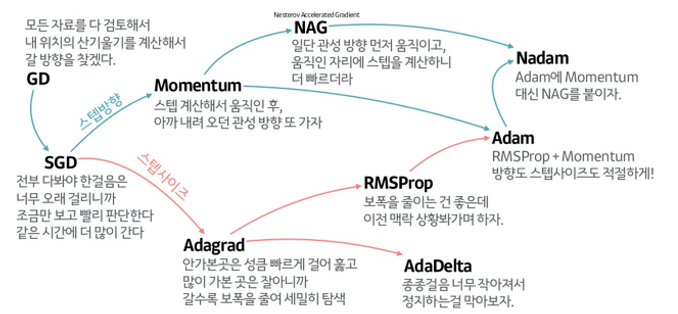

# Model Set-up
autoencoder = Model(inputs=encoder.input, outputs=decoder(encoder.output))
autoencoder.compile(loss='mean_squared_error', optimizer='adam')

plt.figure(figsize=(40,100))
model_history = autoencoder.fit(x_train, x_train, epochs=50, batch_size=100, verbose=0,
                                callbacks=[TestEncoder(x_train[0:500], y_train[0:500])])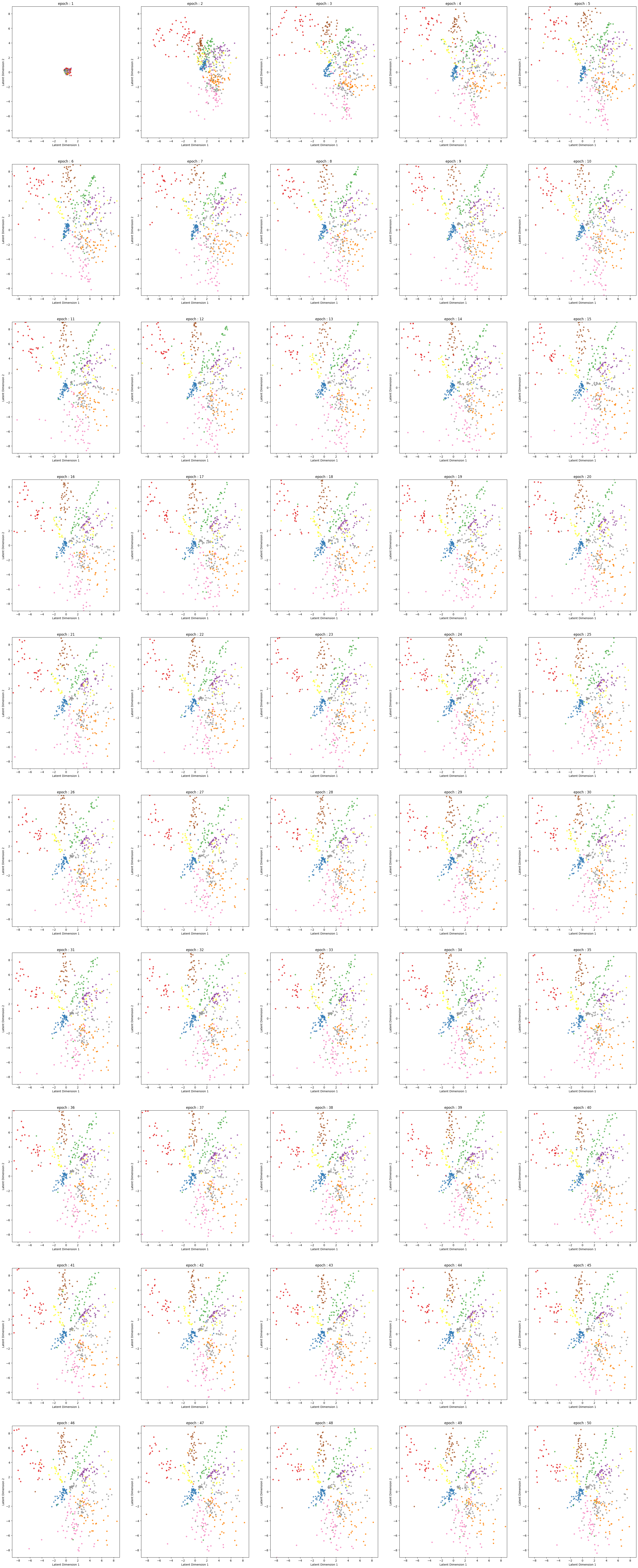

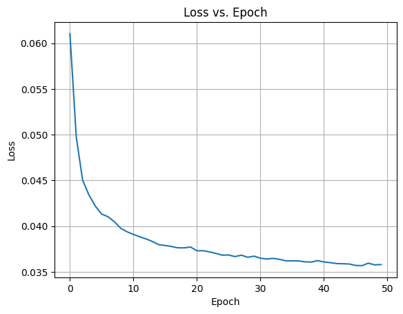
plt.plot(model_history.history["loss"])
plt.title("Loss vs. Epoch")
plt.ylabel("Loss")
plt.xlabel("Epoch")
plt.grid(True)