Machine learing - sklearn 실습

1. Import the NumPy library to create a 3x3 matrix with values ranging 0-8. The expected output should look as follows:
array([[10, 11, 12],
[13, 14, 15],
[16, 17, 18]])

A.

import numpy as np

A = np.array([[0,1,2],[3,4,5],[6,7,8]])
A

2. Use create a 2x2 NumPy array with random values drawn from a uniform distribution using the random seed 123 and show the results below.

A.

rng = np.random.RandomState(123)
rng.uniform(0.0,1.0,4).reshape(2,2)

3. Given an array A,

array([[ 1, 2, 3, 4],
[ 5, 6, 7, 8],
[ 9, 10, 11, 12],
[13, 14, 15, 16]])

use the NumPy slicing syntax to only select the 2x2 lower-right corner of this matrix.

A.

A = np.array([
    [1, 2, 3, 4],
    [5, 6, 7, 8],
    [9, 10, 11, 12],
    [13, 14, 15, 16]])

A[-2:,-2:]

4. Given the array A below, find the least frequent integer in that array:
rng = np.random.RandomState(123)
A = rng.randint(0, 10, 200)
counts = np.bincount(A)

A.

np.argmin(counts)

5. Complete the line of code below to read in the 'train_data.txt' dataset, which consists of 3 columns: 2 feature columns and 1 class label column. The columns are separated via commas and show the first 5 lines of the DataFrame.

A.

import pandas as pd

df_train = pd.read_csv('train_data.txt',sep = ',')
df_train.head()

6. Consider the following code below, which plots one the samples from class 0 in a 2D scatterplot using matplotlib:

X_train = df_train[['x1', 'x2']].values
y_train = df_train['y'].values
%matplotlib inline
import matplotlib.pyplot as plt


plt.scatter(X_train[y_train == 0, 0],
            X_train[y_train == 0, 1], 
            label='class 0',)

plt.xlabel('x1')
plt.ylabel('x2')
plt.xlim([-20, 20])
plt.ylim([-20, 20])
plt.legend(loc='upper left')
plt.show()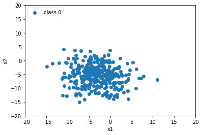

A.

plt.scatter(X_train[y_train == 0, 0],
            X_train[y_train == 0, 1], 
            label='class 0',)

plt.scatter(X_train[y_train == 1, 0],
            X_train[y_train == 1, 1], 
            label='class 1',)

plt.xlabel('x1')
plt.ylabel('x2')
plt.xlim([-20, 20])
plt.ylim([-20, 20])
plt.legend(loc='upper left')
plt.show()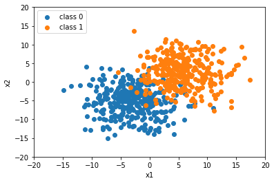

7. Consider the we trained a 3-nearest neighbor classifier using scikit-learn on the previous training dataset:

from sklearn.neighbors import KNeighborsClassifier

knn = KNeighborsClassifier(n_neighbors=3)
knn.fit(X_train, y_train)

from mlxtend.plotting import plot_decision_regions

plot_decision_regions(X_train, y_train, knn)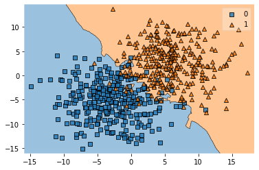

A.

errors = int(len(y_train) - knn.score(X_train, y_train) *len(y_train))
errors

8. Use the code from E 7) to also visualize the decision boundaries of k-nearest neighbor classifiers with k=1, k=5, k=7, k=9 compute the prediction error on the training set for the k-nearest neighbor classifiers with k=1, k=5, k=7, k=9

A.

knn = KNeighborsClassifier(n_neighbors=1)
knn.fit(X_train, y_train)
plot_decision_regions(X_train, y_train, knn)
errors = int(len(y_train) - knn.score(X_train, y_train) *len(y_train))
print('Errors:', errors)

knn = KNeighborsClassifier(n_neighbors=5)
knn.fit(X_train, y_train)
plot_decision_regions(X_train, y_train, knn)
errors = int(len(y_train) - knn.score(X_train, y_train) *len(y_train))
print('Errors:', errors)

knn = KNeighborsClassifier(n_neighbors=7)
knn.fit(X_train, y_train)
plot_decision_regions(X_train, y_train, knn)
errors = int(len(y_train) - knn.score(X_train, y_train) *len(y_train))
print('Errors:', errors)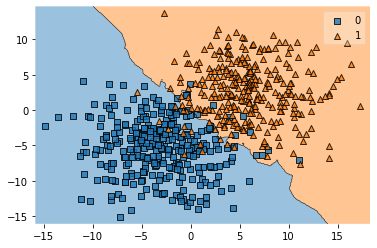

knn = KNeighborsClassifier(n_neighbors=9)
knn.fit(X_train, y_train)
plot_decision_regions(X_train, y_train, knn)
errors = int(len(y_train) - knn.score(X_train, y_train) *len(y_train))
print('Errors:', errors)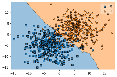

9. Using a similar approach you used in E 5), now load the test_data.txt file into a pandas array. However, note that the dataset now has whitespaces separating the columns instead of commas.

A.

df_test = pd.read_csv('test_data.txt',sep = " ")

df_test.head()

X_test = df_test[['x1', 'x2']].values
y_test = df_test['y'].values

10. Use the train_test_split function from scikit-learn to divide the training dataset further into a training subset and a validation set. The validation set should be 20% of the training dataset size, and the training subset should be 80% of the training dataset size.
For you reference, the train_test_split function is documented at http://scikit-learn.org/stable/modules/generated/sklearn.model_selection.train_test_split.html.

A.

from sklearn.model_selection import train_test_split


X_train_sub, X_val, y_train_sub, y_val = train_test_split(X_train, y_train,
                                                          test_size=0.2,
                                                          random_state =123,
                                                          stratify=y_train)

11. Write a for loop to evaluate different k nn models with k=1 to k=14. In particular, fit the KNeighborsClassifier on the training subset, then evaluate it on the training subset, validation subset, and test subset. Report the respective classification error or accuracy.

A.

df_test = pd.read_csv('test_data.txt',sep = " ")
X_test = df_test[['x1', 'x2']].values
y_test = df_test['y'].values


for k in range(1, 15):
    knn = KNeighborsClassifier(n_neighbors=k)
    knn.fit(X_train_sub, y_train_sub)
    y_pred = knn.predict(X_test)
    num_correct_predictions = (y_pred == y_test).sum()
    accuracy1 = knn.score(X_train_sub,y_train_sub) * 100
    accuracy2 = knn.score(X_val,y_val) * 100
    accuracy3 = (num_correct_predictions / y_test.shape[0]) * 100
    print("k = ",k,f'Train set accuracy: {accuracy1:.2f}%',f'Val set accuracy: {accuracy2:.2f}%',f'Test set accuracy: {accuracy3:.2f}%')