Logistic Regression is commonly used to estimate the probability that an instance belongs to a particular class. If the estimated probablility is greater than 50%, then the model predicts that the instance belongs to that class (called the positive class, labeled "1"), or else it predicts that it does not (it belongs to the negative class, labeled "0"). This makes it a binary classifier.
-> Logistic "Regression"은 회귀 방식을 사용하지만, estimated probability의 수치가 50% 이상이면 1로, 나머지는 0으로 분류 작업을 수행한다.
1) probability & prediction
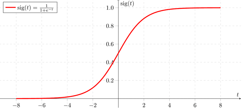
linear regression과 마찬가지로 logistic regression도 input값에 weight를 곱한 뒤 이들을 bias와 더한 형태를 가지는데, 식의 결과값을 directly 반환하는 linear regression과 다르게 logistic regression은 logistic 함수 에 이 결과값을 넣은 값을 반환한다. logistic이 곧 sigmoid 이므로, 최종 output은 0과 1사이의 값을 갖는다.
-
estimated probability
-
logistic function
logistic regression 모델로 instance 가 positive class에 속할 확률 을 구했다면, prediction 는 아래와 같이 구할 수 있다.
- model prediction
또한, , 이므로 logistic regression 모델은 가 음수일 때 0으로, 양수일 때 1로 예측하게 된다.
*score 는 logit이라고도 불린다. estimated probability 를 logit function, 에 넣은 결과가 기 때문. logit은 positive class에 대한 probability와 negative class에 대한 probability의 비율의 log이므로 log-odds라고도 한다.
2) training & cost function
training의 목적은 positive instance(y=1)인 경우 높은 prob를, negative instance(y=0)인 경우 낮은 prob를 갖는 parameter vector 를 설정하는 것이다. 이는 cost function 을 통해 설명될 수 있다.
- cost function
아래의 그래프에서 x는 0에 가까워질수록 는 커진다. 이는 positive instance에 대한 prob가 0에 가까울수록 cost가 커지는 것을 의미한다. 반대로 x가 1에 가까워질수록 는 커진다. 이는 negative instance에 대한 prob가 1에 가까울수록 cost가 커지는 것을 의미한다.
가 1일 때 는 0이라는 건 positive instance의 prob가 1일 때 cost가 0임을, 가 0일 때 가 0이라는 건 negative instance의 prob가 0일 때 cost가 0임을 의미한다.
whole training set에 대한 cost function은 모든 training instances에 대한 비용을 평균한 것이다. 이는 log loss라고 불린다.
- cost function, log loss
에 대한 cost function을 최적화하는 closed-form 방정식은 없지만, cost function이 convex하기 때문에 gradient descent와 같은 최적화 알고리즘을 이용하여 global minimum을 구할 수는 있다.
j번째 model parameter 에 대한 cost function의 편미분을 구하면 각 instance에 대한 prediction error와 j번째 feature value의 곱을 모두 더한뒤 평균을 낸 것과 같음을 알 수 있다.
- cost function derivatives
모든 partial derivatives를 포함하는 gradient vector를 구한 다음에는 Batch GD, Stochastic GD, Mini-batch GD 등으로 최적화하면 된다.
3) decision boundaries
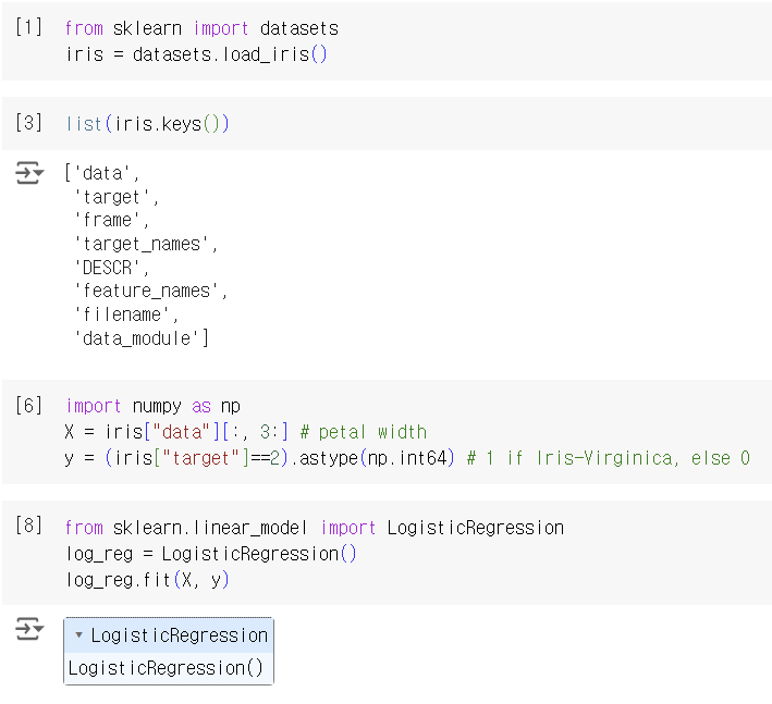
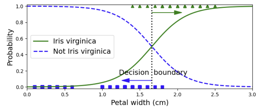
Iris는 Virginica, Versicolor, Setosa 총 3종이 있는데 여기서는 Iris-Virginica를 petal width라는 하나의 feature로만 분류하려고 한다.
모델 학습 결과로 estimated probabilities를 확인할 수 있다. Iris-Virginica는 1.4 ~ 2.5 구간에, Not Iris-Virginica는 0.1 ~ 1.8 구간에 존재한다. 2이상의 구간에서는 확실하게 Iris-Virginica로 분류되며 1이하의 구간에서는 확실하게 Not Iris-Virginica로 분류된다. 그 사이의 구간에서는 overlap이 발생한 것으로 보아 classifier가 불확실함을 볼 수 있다.
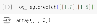
probability를 반환하는 predict_proba 대신 예측 class를 반환하는 predict 메서드를 사용하면 결정 경계를 구할 수도 있는데 1.7와 1.5을 넣었을 때 각각 1과 0을 반환한 것으로 보아, 결정 경계가 1.6 근처 어딘가에 있음을 알 수 있다. 참고로 decision boundary는 0과 1의 probability 모두 50%로 동일한 지점을 말한다.
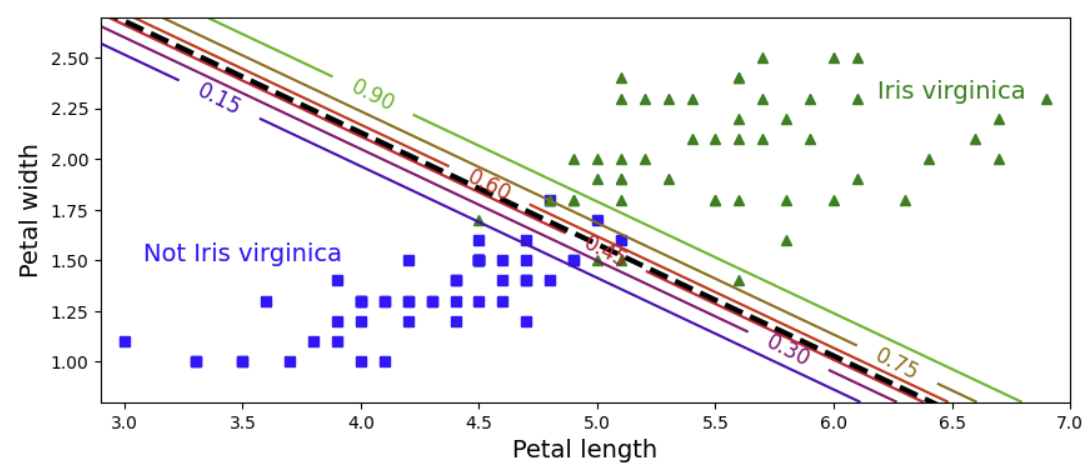
이번에는 petal width와 length로 분류를 하였다. 점선은 모델이 probability를 50% 예측한 지점이며 곧 decision boundary이다. 그리고 이와 평행한 선들은 아래부터 probability가 15% ~ 90%인 지점을 나타낸다.
다른 linear model들과 마찬가지로 logistic regression도 과 penalty로 regularized 될 수 있다. scikit learn의 default는 이다. 다른 linear model에서는 regularization의 강도를 조절하는 hyperparameter로 alpha를 사용하지만, logistic regression은 역수인 C를 사용한다. 그래서 C가 커지면 모델이 정규화되는 정도가 작아진다.
4) softmax regression
앞에서 binary classifier가 multiple class를 분류하려면 분류기를 여러개 combine 해야 했다. 그런데 logistic regression은 direct하게 multiclass classification을 할 수 있으며, 이를 softmax regression 또는 multinomial softmax regression이라고 한다.
4-1) probability & prediction
다중 분류를 하는 과정을 알아보자. 먼저 주어진 instance x에 대해 모든 class의 score를 계산한다. 각 class는 parameter vector 를 가지며 이 벡터들은 parameter matrix 에 저장된다.
- softmax score for class k
x에 대해 모든 class의 score를 계산했다면, score들을 softmax function 에 넣어, x가 각 class에 속할 probability 를 예측할 수 있다. 확률은 class k의 exponential을 sum of all the exponentials로 나누어 normalize한 것으로 나타낼 수 있다.
아래의 수식에서 K는 class의 수, 는 instance x에 대한 각 class의 score들을 담은 벡터, 는 x가 class k에 속할 확률을 의미한다.
- softmax function
logistic regression classifier와 마찬가지로 softmax regression도 가장 높은 probability를 가진 class를 output class로 예측한다. argmax 연산자를 이용하면 최대값을 갖는 인덱스(클래스)를 찾을 수 있다. *argmax는 argument(인자) of maximum을 의미
- softmax regression classifier prediction
4-2) training & cross entropy
training의 목적은 target class에 대해 높은 probability를 estimate하는 (그리고 나머지에 대해서는 낮은 probability를 estimate하는) 모델을 만드는 것이다. 앞의 logistic regression에서 했듯, cost function을 구하고 GD 방식으로 최적화하면 된다.
softmax function은 cross entropy cost function 을 사용한다. 이는 estimated class probabilities 가 target classes 와 얼마나 잘 매치되는지 확인할 수 있다.
는 i번째 instance가 class k에 속할 확률을 의미하며, 대부분 0 또는 1에 속한다.
- cross entropy cost function
에 대한 cost function의 gradient vector는 다음과 같다. 이를 통해 모든 class의 gradient vector를 계산하고 GD를 이용하여 cross entropy cost function을 최적화하기 위한 parameter matrix 를 찾으면 된다.
- cross entropy gradient vector for class k
4-3) decision boundaries
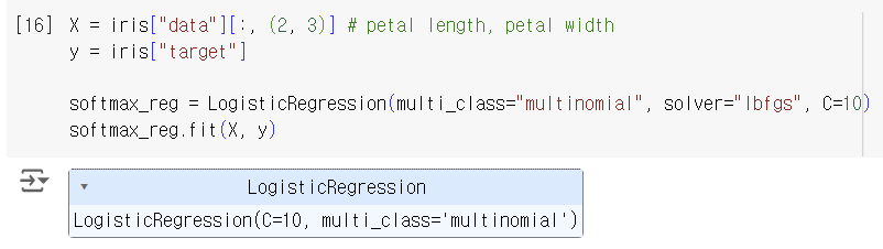
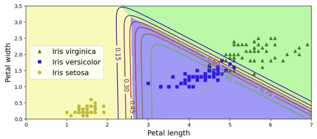
이번에는 Iris 3종을 분류하려고 한다. logistic regression을 multiclass classifier로 그냥 사용하면 OvA 방식으로 진행하겠지만, multi_class hyperparameter를 multinomial로 설정하면 softmax regression을 사용할 수 있다.
logistic regression은 cost function을 최소화하기 위해 최적화 알고리즘을 사용해야 하며, 이때 solver 파라미터가 어떤 최적화 알고리즘을 사용할지 결정한다. solver의 종류에는 아래와 같은 것들이 있지만, 여기서는 다중 분류 문제에 적합한 lbfgs를 사용한다.
- liblinear
- newton-cg
- lbfgs
- sag
- saga
여기서도 regularization을 default로 이용하고, 강도는 C로 조절할 수 있다.
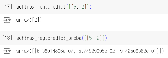
petal length가 5, width가 2인 iris를 예측하면 class 2(Iris-Virginica)가 나오고, class마다 estimated probability를 확인하면 class 2가 94.2%인 것을 확인할 수 있다.
이를 시각화하면 다음과 같다. 두 class 간의 경계는 linear한 것을 확인할 수 있다.
plot 그리는 코드 출처2
출처: Hands-On Machine Learning by Aurelien Geron
