Towards Robust Monocular Depth Estimation: Mixing Datasets for Zero-shot Cross-dataset Transfer 논문 리뷰

신희준·2024년 2월 16일

Paper Review

목록 보기

22/28

Paper : Towards Robust Monocular Depth Estimation: Mixing Datasets for Zero-shot Cross-dataset Transfer (René Ranftl, Katrin Lasinger, David Hafner, Konrad Schindler, Vladlen Koltun / IEEE PAMI 2022)

Intel lab에서 발표한 monocular depth estimation 연구로, 서로 다른 bias를 가진 여러 데이터 셋을 함께 학습시킴으로써 다양한 환경에서 촬영된 한번도 보지 못한 scene의 single image에 대한 depth estimation을 robust하게 수행할 수 있게 하였다.

단순히 technical novelty가 있는 연구보다도 실제 application에 다양하게 활용될 수 있다는 데에 의의가 있다고 생각한다.

Intel Technology MiDaS demo video

https://www.youtube.com/watch?v=D46FzVyL9I8

Highlights

Occlusion을 robust하게 다루기 위한 minimum reprojection loss
Visual artifact를 줄이기 위한 full-resolution multi-scale sampling method
Camera motion 가정을 해치는 training pixel을 무시하기 위한 auto-masking loss

Introduction

Depth는 physical environment를 이해하기 위한 아주 강력한 representation으로, learning-based monocular depth estimation을 위한 많은 연구가 진행되었다.

Machine-learning 기반의 monocular depth estimation의 가장 어려운 점은 바로 충분한 학습 데이터를 확보하기 어렵다는 것이다.

학습에 사용되는 depth map을 얻는 sensor나 method로는 structured light, time-of-flight sensors, laser scanners, stereo cameras, structure-from-motion (SfM) 등이 있는데, 이러한 data들은 충분히 많은 양을 얻기 어려울뿐더러 각각의 source로부터 얻은 데이터는 이미지가 얻어지는 방식에 따라 bias가 존재하기 때문에, 다양한 scene의 실제 image에 robust하게 작동하는 모델을 만드는 데에는 여전히 어려움이 있다.

이러한 문제를 해결하기 위해서 이 논문에서는 데이터셋 사이의 incompatibility를 여러 요인 (unknown, inconsisent scale 등)에 invariant한 loss function을 개발하여, 다양한 sensing modalities (stereo cameras, laser scanners 등)에서 얻어진 데이터를 함께 학습시킬 수 있는 방법을 제안하였다.

추가적으로, 이렇게 다양한 데이터를 함께 학습하는 최적의 strategy를 제안하며, 많은 실험을 통해 다양한 source에서 얻어진 image에 대해 매우 좋은 성능을 보여주었다.

여기서 zero-shot cross-dataset transfer라는 용어를 사용하는데, 이는 특정 데이터셋에 대해 학습하고, 학습 시에 보지 못한 test dataset에 대해 성능을 측정하는 것을 의미한다 (학습에 사용된 데이터 셋의 subset을 testing으로 쓰지 않는다는 것을 의미; 완전히 다른 source의 데이터 셋).

당연하게도, 이런 zero-shot cross-dataset 성능은 우리가 학습한 모델의 "real world" 성능을 반영하게 된다.

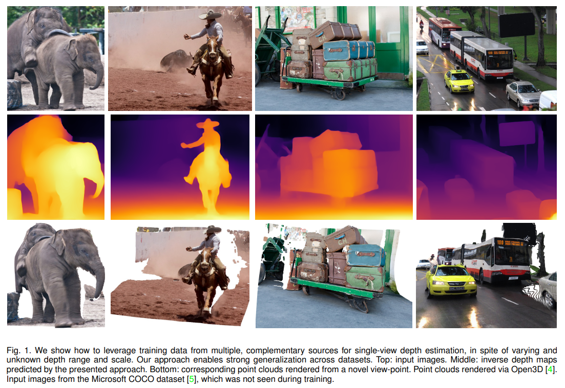
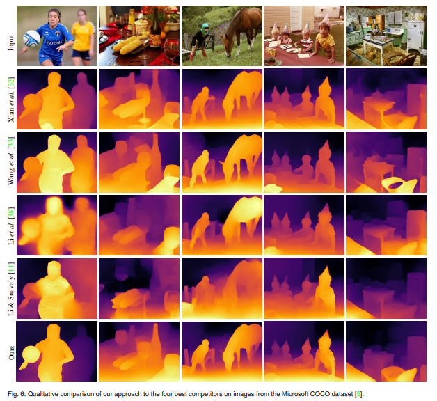
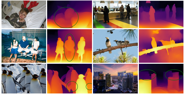
아래의 예시도 Microsoft COCO dataset 이미지를 inference한 결과로, 학습에 아예 사용되지 않은 이미지들이다.

Existing Datasets

해당 논문이 다양한 데이터셋의 mixing strategy에 관련된 만큼, monocular depth estimation에서 주로 사용되는 데이터셋을 알아보자.

보통 데이터셋은 RGB image와 이에 상응하는 depth annotation으로 이루어져 있으며, dataset들은 촬영한 environment나 object (indoor/outdoor scenes, dynamic objects), depth annotation의 종류 (sparse/dense, absolute/relative depth), accuracy (laser, time-of-flight, SfM, stereo, human annotation, synthetic data), image quality와 camera setting, 그리고 dataset size 등이 서로 다르다.

각 dataset은 고유한 특성과 bias를 가지고 있기 때문에, 하나의 dataset에서 학습한 모델은 같은 dataset (같은 camera parameters, depth annotation, environment)에 대한 test split에는 잘 작동하겠지만, 다른 특성을 가지는 unseen data로 generalize되기 힘들 것이다.

이 논문에서는 다양한 training dataset을 함께 학습시키는 방법을 제안하고 이것이 강력한 generalization capability로 이어진다는 것을 보여주었다.

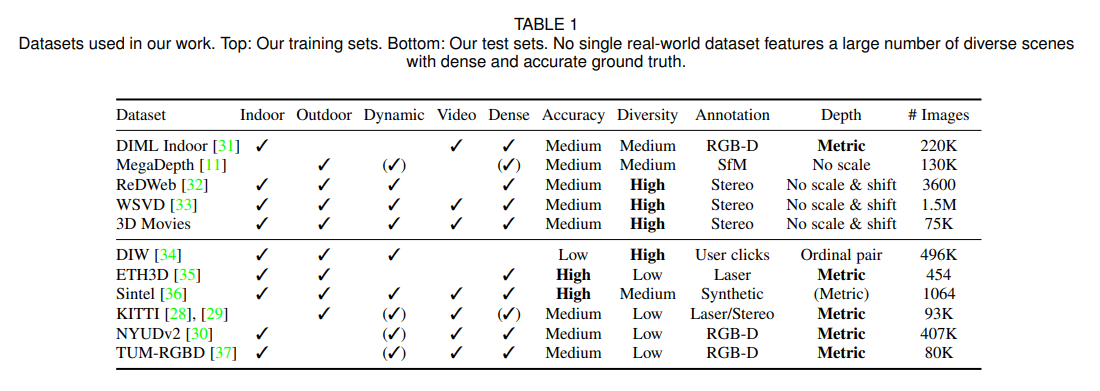
아래의 표에서 이 연구에 사용된 5개의 training와 5개의 testing dataset를 확인할 수 있다.

Training datasets

ReDWeb (RW) : 상대적으로 큰 stereo baseline으로 얻어진 ground truth가 있는 데이터로, 크기가 작지만 diverse & dynamic한 scene이 포함된 매우 선별된 작은 dataset
MegaDepth (MD) : wide-baseline multi-view stereo reconstruction으로 얻어져서 background region이 더욱 정확한 ground truth가 있는 데이터로, 훨씬 많은 이미지가 있지만 대부분 static scene
WSVD (WS) : web에서 얻어진 stereo video로 이루어진 dataset으로, diverse & dynamic scene이 포함. (Ground truth가 같이 제공되는 데이터셋은 아니므로 해당 데이터셋 공개한 저자의 방식을 따라서 생성)
DIML Indoor (DL) : static indoor scene으로 이루어진 RGB-D로 얻어진 dataset

Testing datasets

DIW : 매우 다양하지만 sparse ordinal relation 형태의 ground truth만을 제공
ETH3D : static scene에 대해 매우 정확한 laser-scanned ground truth 제공
Sintel : synthetic scene에 대해 완벽한 정확도의 ground truth 제공
KITTI & NYU : depth estimation에서 자주 사용되는 dataset
TUM : indoor enviroment의 dynamic subset을 사용

위의 6개 데이터셋에 대해서는 fine-tuning을 하지 않았기 때문에 이를 zero-shot cross-dataset transfer라고 한다.

3D Movies

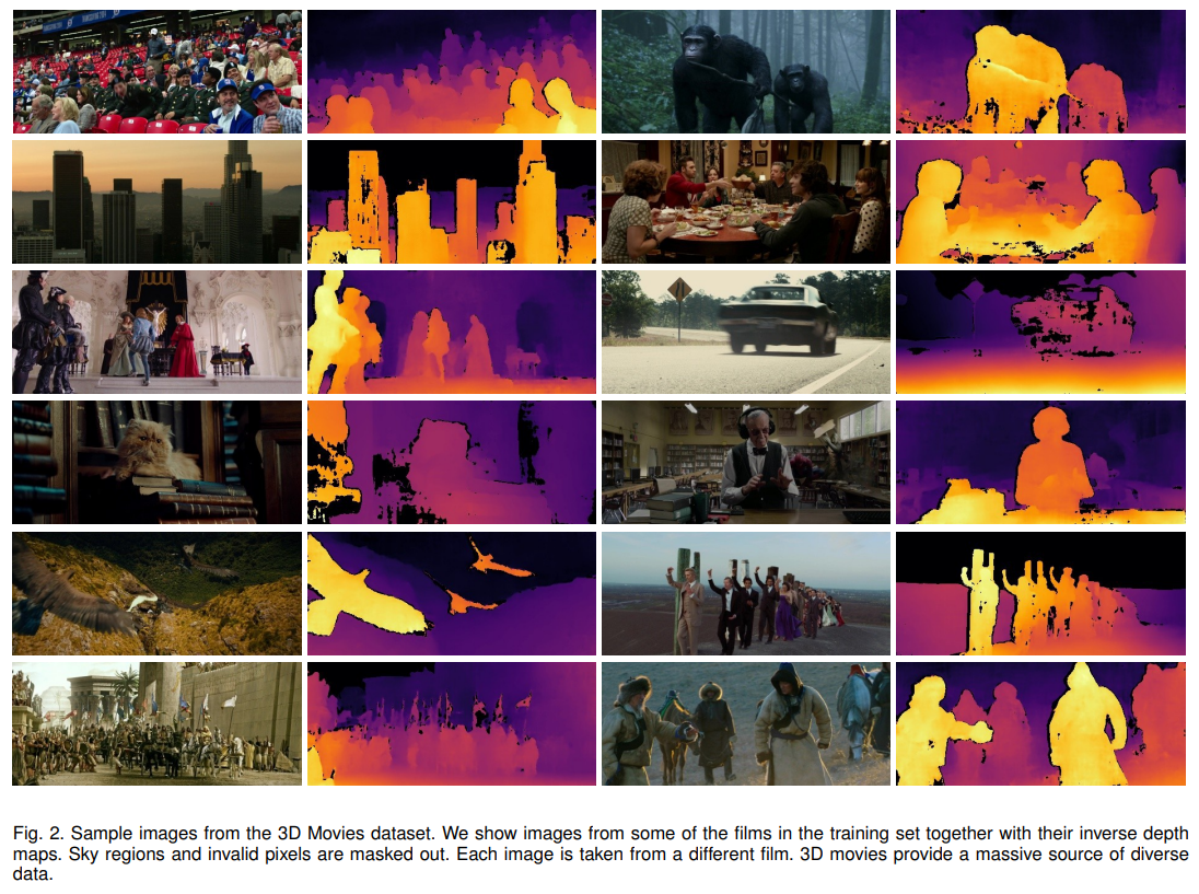
저자들은 기존의 데이터에 추가적으로 3D movies (MV) dataset을 제시하였다.

3D movies dataset은 매우 다양한 source에서 촬영된 dynamic environment에 대한 high-quality video frames이 포함된 데이터셋이다.

이 데이터들은 metric depth를 제공하지는 않기 때문에, 상대적인 depth를 얻기 위해 stereo matching 기법을 사용하였다.

3D movie dataset는 아주 잘 control된 condition에서 촬영된 stereo pair를 제공한다 장점이 있는 반면에, 하나의 영화 내부에서도 여러 가지 요인에 의해 촬영 조건이 조금씩 바뀔 수 있다는 단점이 있다. 예를 들어서, 영화에서 stereographer들은 영화 초기에는 흥미를 불어일으키기 위해 매우 입체적인 효과를 내기도하고 (disparity range를 늘린다), 영화 중간에는 편안한 시청을 위해 depth budget를 줄이기도 한다.

결과적으로 한 영화 안에서도 focal lengths, baseline, convergence angle 등이 계쏙 변화할 수 있다. 게다가 일반적인 stereo camera와 다르게 영화 촬영에서 stereo pair에서는 물체가 screen 앞에나 뒤에 있는 것으로 인식될 수 있게 하기 위해 postive, negative disparity가 둘 다 존재할 수 있다. 추가적으로, depth는 영화 내의 각 scene dependent하고, post-production을 통해 바뀔 수 있다.

이 논문에서는 23개의 영화를 선택하고, processing하여 frame을 선택하고 stereo matching을 통해 disparity map을 추출하였다. (자세한 과정은 생략)

Training on Diverse Data

Monocular depth estimation training에서 다양한 데이터를 사용하는데 가장 어려운 점은 바로 ground truth가 서로 다른 form으로 존재한다는 것이다.

예를 들어, laser-based measurement나 calibration을 아는 stereo camera는 absolute depth를, SfM은 unknown scale의 depth를, calibration을 모르는 stereo camera는 disparity map의 형태로 ground truth가 주어진다.

Diverse source로부터 주어지는 다양한 ground truth 정보를 최대한 잘 활용하면서 training하기 위해서는 아래의 3가지 문제를 풀어야한다.

서로 다른 Depth representation
Direct depth vs. Inverse depth representation
Scale ambiguity
어떤 dataset은 depth가 unknown scale로 주어진다
Shift ambiguity
어떤 dataset은 disparity의 scale과 global disparity shift에 대한 정보가 없다. (global disparity shift란 disparity로부터 depth를 구할 때 사용되는, baseline이나 principle point를 모르거나, 어떤 processing으로 인해 변하였을 때 고려하는 것이라고 생각하면 된다.)

Scale- and shift-invariant losses

본 논문에서는 위에서 언급한 문제를 해결하기 위하여 scale/shift invariant loss를 제안하였으며, disparity space (scale과 shift에 영향을 받지 않는 inverse depth)에서 model prediction을 수행하였다.

$M$ 개의 pixel을 가진 image가 주어졌을 때, parameter $\theta$ 를 갖는 prediction model이 disparity prediction $d=d(\theta) \in \mathbb R^M$ 을 예측하고, $d^* \in \mathbb R^M$ 을 상응하는 GT disparity라고 하자.

그러면 하나의 이미지에 대해 scale- and shift-invariant loss는 아래와 같이 정의한다.

\mathcal L_{ssi}(\hat{d},\hat{d}^*)=\frac{1}{2M}\sum^m_{i=1}\rho (\hat{d_i},\hat{d_i^*})

여기서 $\hat{d}$ 와 $\hat{d^*}$ 는 prediction과 ground truth가 scale & shift된 것이고, $\rho$ 는 특정 형태의 loss function (L1/L2 등)을 의미한다.

그런데, 이 scale과 shift으로 어떻게 해줘야할까?

이제, $s:\mathbb R^M\to\mathbb R_+$ 을 scale estimator, $t:\mathbb R^M\to\mathbb R$ 를 translation estimator라고 하자. (=function)

Scale & shift invariant loss가 잘 작동하기 위해서는 pred와 gt가 각각의 scale과 shift에 대해 align되어야 한다. (i.e., $s(\hat{d}) \approx s(\hat{d^*})$ , $t(\hat{d}) \approx t(\hat{d^*})$ )

Align을 위해서 저자들은 두 가지 방법을 제안하였다.

1) Least-squares criterion을 통해 prediction을 scale & shift하여 ground truth로 align하는 방식

(s,t)=argmin_{s,t}\sum^M_{i=1}(s\bold{d}_i+t-\bold{d}_i^*)^2

\bold{\hat{d}}= s\bold{d}+t, \quad \bold{\hat{d^*}}=\bold{d^*}

여기서 $\bold{\hat{d}}$ 와 $\bold{\hat{d^*}}$ 는 align된 prediction과 ground truth이다.

$s$ 와 $t$ 는 위의 식을 아래와 같은 standard least-squares problem으로 쓸 수 있는데,

\bold{h}^{opt}=argmin_h\sum^M_{i=1}(\bold{\vec{d}}_i^T\bold{h}-\bold{d}_i^*)

\bold{\vec{d}}_i=(\bold{d}_i,1)^T, \bold{h}=(s,t)^T

이는 closed-form solution을 갖는다. (위의 식 $h$ 에 대해서 미분)

\bold{h}^{opt}=(\sum^M_{i=1}(\bold{\vec{d}}_i\bold{\vec{d}}_i^T))^{-1}(\sum^M_{i=1}(\bold{\vec{d}}_i\bold{{d}}_i^*))

$\bold{h}^{opt}=(s^{opt}, t^{opt})$ 를 구하고 나면, 이 scale과 shift를 model output $\bold{d}$ 에 적용하여 aligned prediction $\bold{\hat{d}}$ 를 구한다. (ground truth disparity는 $\bold{\hat{d^*}}=\bold{d^*}$ 로 설정 되어 있으므로 이 두 값을 이용해 loss 구하면 된다.)

이제, loss function $\rho(x)=\rho_{mse}(x)=x^2$ 로 설정하면, 이제 scale & shift invariant mean-squared error $\mathcal L_{ssimse}$ 를 정의할 수 있다.

하지만, 기존의 large-scale의 training dataset들이 imperfect ground truth를 가지고 있다는 점을 감안하면, outlier에 취약한 MSE보다는 조금 더 robust한 loss function이 필요하다.

2) Robust estimator를 이용하여 prediction과 ground truth를 함께 scale & shift하여 align하는 방식

t(\bold{d})=median(\bold{d}), \quad s(\bold{d})=\frac{1}{M}\sum^M _{i=1}|\bold{d}-t(\bold{d})|

이를 이용하여 pred와 gt가 zero-translation과 unit scale을 가지도록 align시킨다.

\bold{\hat{d}}=\frac{\bold{d}-t(\bold{d})}{s(\bold{d})}, \quad \bold{\hat{d}^*}=\frac{\bold{d}^*-t(\bold{d}^*)}{s(\bold{d}^*)}

$\rho_{mae}(x)=|x|$ 로 설정하면 robust loss $\mathcal L_{ssimae}$ 를 정의할 수 있다.

추가로 모든 image에 상위 20%의 residual을 갖는 pixel에 대한 영향을 제거하는데, 이는 gt의 outlier가 학습에 주는 영향을 없애기 위함이라고 한다.

\mathcal L_{ssimtrim}(\bold{\hat{d}},\bold{\hat{d}}^*)=\frac{1}{2M}\sum^{U_m}_{j=1}\rho_{mae}(\bold{\hat{d}}_j-\bold{\hat{d}}_j^*)

여기서 $|\bold{\hat{d}}_j-\bold{\hat{d}}_j^*| \le |\bold{\hat{d}}_{j+1}-\bold{\hat{d}}_{j+1}^*|$ 이고, $U_m=0.8M$

Scale & shift invariant loss는 이전의 많은 연구에서 논의된 loss들에 비해 몇 가지 장점을 갖는다.

Scale & shift invariant loss는 scale과 shift에 대한 정보가 없이도 여러 데이터셋에 대해 직접적으로 loss calculation이 가능하다.

이 loss는 disparity space에서 정의가 되었기 때문에 수치적으로 stable하기 때문에 학습이 용이하고, 다양한 depth representation으로 적용될 수 있는 장점이 있다.

Final Loss

최종 loss에는 disparity space에 대한 multi-scale, scale-invariant gradient matching term을 추가로 사용한다. 이 loss는 disparity의 discontinuity가 ground truth와 비슷해지도록 한다.

\mathcal L_{reg}(\bold{\hat{d}},\bold{\hat{d}}^*)=\frac{1}{M}\sum^K_{k=1}\sum^M_{i=1}(|\nabla_xR^k_i|+|\nabla_yR^k_i|)

여기서 $R_i=\bold{\hat{d}}_i-\bold{\hat{d}}_i^*$ 이고, $R^k$ 는 scale $k$ 에서의 disparity map difference. ( $k$ 는 image resolution scale을 의미하며 4개 scale 사용)

그러면 training set $l$ 에 대한 최종 training loss는 아래와 같다.

\mathcal L_l=\frac{1}{N_l}\sum^{N_l}_{n=1}\mathcal L_{ssi}(\bold{\hat{d}}^n, \bold{(\hat{d}^*})^n)+\alpha\mathcal L_{reg}(\bold{\hat{d}}^n, (\bold{\hat{d}^*})^n)

Mixing Strategy

위에서 정의한 loss에 더불어서, 서로 다른 데이터셋을 어떤 식으로 조합해서 학습을 해야 할지에 대해 2가지 전략을 제안하였다.

1) Naive Strategy

단순한 mixing strategy로는 batch 내부에 서로 다른 데이터셋의 sample을 균등하게 넣어 학습하는 것이다. 각 dataset의 size와 관계없이, 모든 데이터를 충분히 학습할 수 있게 된다.

2) Pareto-optimal multi-task learning

조금 더 복잡한 방법으로는 각 데이터셋으로 학습하는 것을 분리된 task로 보고, 적당한 Pareto optimum을 찾는 것이다.

Pareto optimum solution은 여러 training set에 대해서 하나의 set에 대한 loss를 increase하지 않고서는 다른 set에 대한 loss를 decrease할 수 없는 점을 뜻한다.

min_{\theta}(\mathcal L_1(\theta),...,\mathcal L_L(\theta))^T

여기서 parameter $\theta$ 는 모든 데이터셋이 공유한다.

Results

참고로 이 연구는 ResNet기반의 multi-scale architecture를 사용하였다.

Loss term ablation

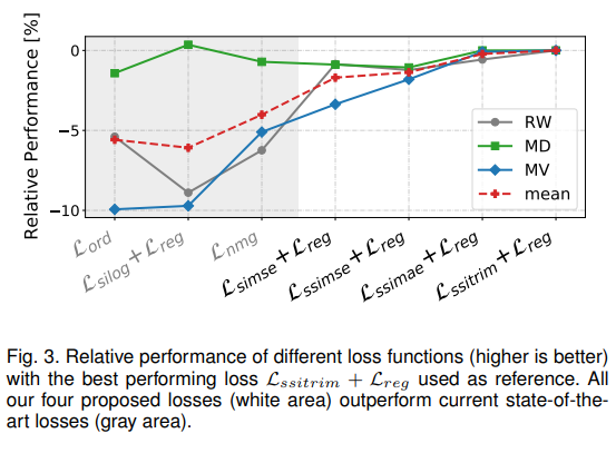
위에서 제안된 많은 loss term에 대해 ablation을 진행하였고, $\mathcal L_{ssitrim}+\mathcal L_{reg}$ 에서 가장 좋은 성능을 보였기 때문에, 이후 모든 실험은 해당 loss를 사용하였다.

Encoder ablation

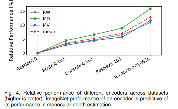
Encoder architecture에 대한 ablation을 진행하였고, high capability의 network를 encoder로 사용할 때 성능이 더욱 좋아진다고 한다. 추가적으로 모든 network는 imagenet pretraining이 되었는데, imagenet training이전에 weakly-supervised data를 통해 pretraining을 해준 network (ResNeXt-101-WSL)가 훨씬 더 좋은 성능을 보여준다고 한다. 이후 모든 실험은 해당 네트워크를 사용하였다.

Dataset ablation

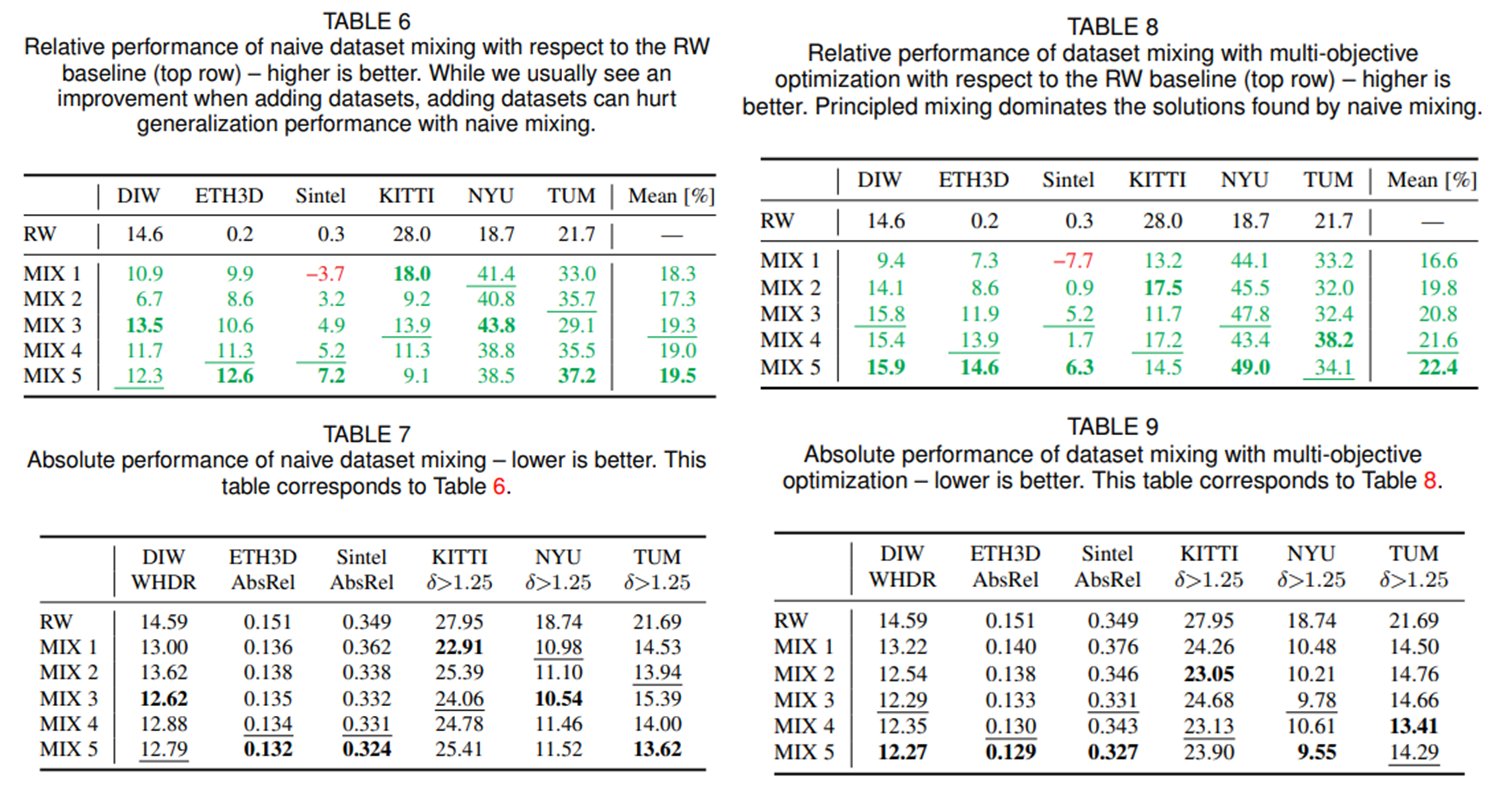
위 table은 dataset mixing에 대한 ablation study에 대한 내용이다. 모든 5가지 데이터를 함께 학습하였을때, 그리고 Pareto-optimal mixing 방법을 사용하였을 때 최고 성능을 보여준다고 한다.

Quantitative & Qualitative results

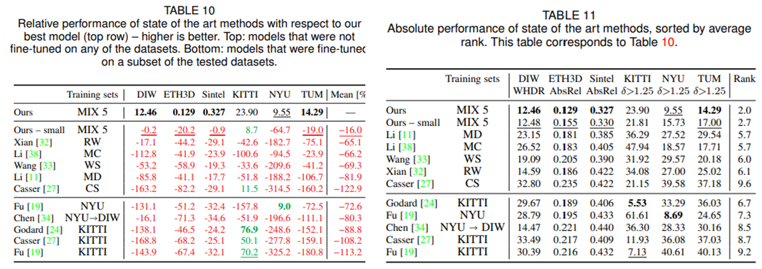
마지막으로 기존의 다른 연구들과의 성능 비교이다. 위의 표에 나타나있는 것 처럼 여러 데이터셋에 대해서 가장 좋은 성능을 보여준다. 특히, 다른 기존 모델들도 특정 데이터 셋으로 finetuning했을 시에는 어느정도 나아진 성능을 보이나, 모든 데이터에 대해 generalize하기에는 여전히 부족하다는 것을 볼 수 있다.

Failure Cases

몇 가지 흥미로운 failure cases도 소개하고 있다. 많은 경우 이미지에서 윗부분이 아랫부분보다 camera로부터 먼 경우가 많기 때문에, 이러한 bias가 모델에도 반영이 되어있다.

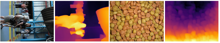
예를 들어 위의 두 예시를 보면 왼쪽의 90도로 회전된 이미지의 땅부분의 깊이를 잘 추정하지 못하고 있고, 오른쪽 이미지에서도 개밥처럼 생긴것들이 사실은 다 같은 거리에 있으나, 아래쪽이 더 가까운 것으로 추정하였다.

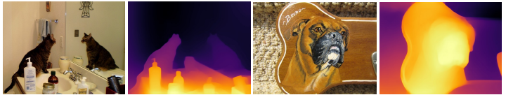
또 다른 예시로는 그림, 사진이나 거울이 있는 이미지의 경우인데, 이미지 내부의 반사체 자체의 깊이보다는 이에 비춘 모습을 바탕으로 깊이를 추정한다.

추가적으로, edge가 너무 강한 경우 깊이를 잘 추정하지 못하는 경우가 있다고 하고, thin structure가 많은 경우, 연속적이지 않은 여러 물체가 겹쳐있는 경우 디테일을 잘 추정하지 못한다고 한다.

Discussion

역시 데이터가 가장 중요하다는 생각을 하게 되는 연구이다. 이 연구는 네트워크보다는 데이터에 대해 유심히 들여다보면서 최대한 많은 정보를 네트워크에게 주려고 하였다.

다른 연구들처럼 엄청 novelty가 있는 method를 제안한 것은 아니지만, deep learning application의 입장에서 매우 실용적인 방향의 연구인 것 같다.

데이터를 잘 처리하고 이해하는 것이 첫번째고, 이를 소화할 수 있는 아키텍처를 디자인하는 일이 다음인 것 같다. Transformer architecture가 multi-modal dataset에 대한 수용을 통해 빠르게 발전할 수 있었던 것과 비슷한 맥락이 아닐까 생각이 든다.

IntelLab의 github에도 https://github.com/isl-org/MiDaS 쉽게 활용할 수 있도록 올라와있고, 실제로 out-of-distribution data에 대해 잘 작동한다.

Absolute Depth

이 연구의 모델의 output은 결국 relative inverse depth이다.

하지만 실제 application에서는 실제 absolute metric depth (m, mm 등으로 표현된)가 필요할 경우가 있다.

이를 위해서는 scale & shift invariant loss에서 정의한 scale $s$ 와 shift $t$ 에 대한 정보가 필요하다.

Inverse\;Depth = s \times output+t

Absolute\;Depth=\frac{1}{Inverse\;Depth}

Unknown $s$ 와 $t$ 의 경우에는 실제 depth map으로 부터 least squared로 구해내서 사용한다고 한다.

y=Ap, \; A=\begin{bmatrix}x,1\end{bmatrix},\;p=\begin{bmatrix}s\\t\end{bmatrix}

신희준

공부하고 싶은 사람

이전 포스트

Attention Is All You Need 리뷰

다음 포스트