
들어가며
석사 졸업 후 그동안 석사과정 중 했던 프로젝트, 기업과제, 논문, 랩세미나, 개인 공부 등을 정리해야겠다 싶어 하나씩 정리하는 중이다.
그 첫번째 과정으로 랩 세미나에서 발표했던 자료를 다시 짚어보며 복습 겸 정리중에 있는데, 밤을 새며 조사하고 준비했던 추억.. 이 새록새록 돋아난다.
랩 세미나 포스팅 순서에도 나름의 이유가 있는데, 내가 연구한 분야는 라이다 캘리브레이션 및 라이다 포인트 클라우드 데이터를 활용한 딥러닝 기반 3D 물체 인식 분야이다. 그렇기에 머신러닝과 점군(포인트 클라우드) 데이터 특성을 이해하기에 기초가 되는 클러스터링 기법부터 조사 했었다. 이후 k-d tree와 다양한 3차원 물체 인식 딥러닝 모델에 대해 조사 및 스터디를 진행하였고 랩세미나에서 발표했었다.
지금 돌아보면 gif 파일도 찾아가며 제일 예쁘게 준비한 자료가 아니였나 싶다.. 개념이 쉬워서 좀 더 정성을 들일 여유가 있었는지도?
해당 포스트에서는 기본적인 클러스터링 기법인 k-means, 계층적 클러스터링, DBSCAN 기법에 대해 소개하며 각각의 디테일한 요소 또한 살펴볼 것이다.
(발표자료를 그대로 가져왔기에 영어 기반이다. 설명이 부족한 부분은 추가로 한국어로 밑에 기술하였다.)
Clustering
- Basically, clustering is an unsupervised learning method, so it learns without a label.
- Clusters are classified based on similarity without knowledge of the samples.
- To evaluate the similarity between clusters, various distance measurement functions are used, for example, Euclidean distance, Mahalanobis distance, Lance-Williams distance, Hamming distance, etc.
k-means
-
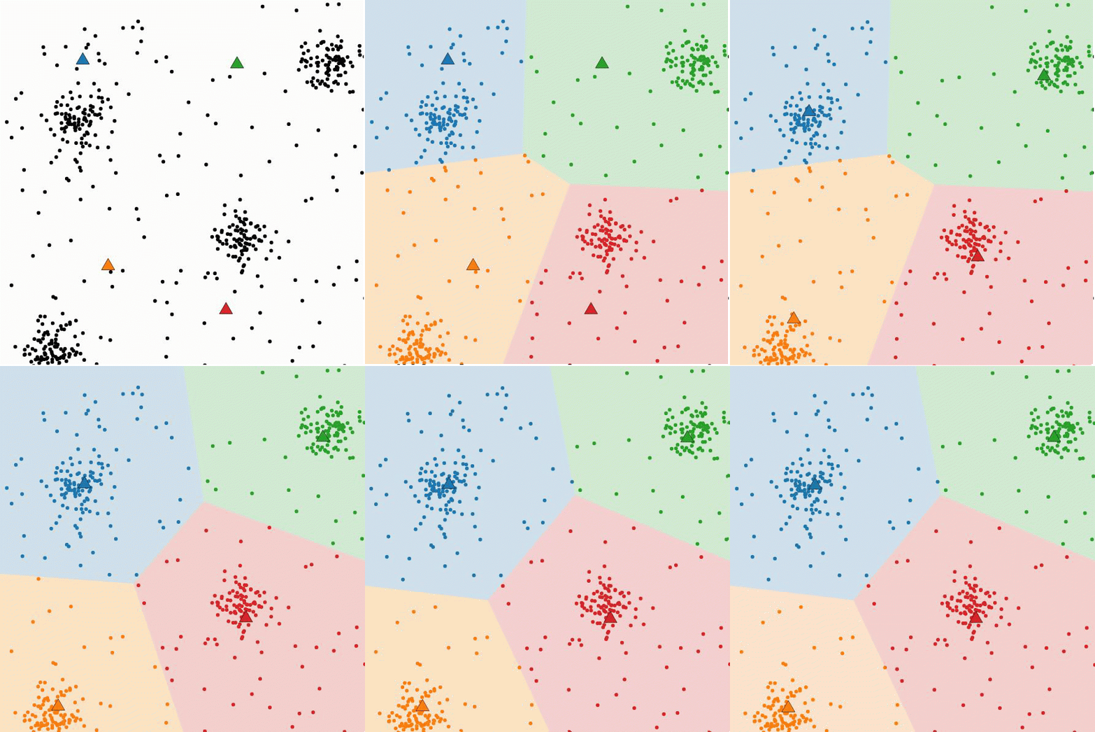
k-means clustering (K=4)
-
위의 그림은 k-means 클러스터링이 진행되는 과정을 보여준다. 자세한 설명은 바로 뒤의 알고리즘 파트에서 설명하겠다.
Algorithm
-
Input
-
K (Number of clusters)
-
Training set
주어진 데이터(Training set)을 K분할로 나누기 위한 입력 값
-
-
Randomly initialize K cluster centroids
-
Cluster indexing
-
Centroid update
Optimization objective
- optimization objective
Objective based clustering
- k-means: Euclidean distance
- k-median: Absolute distance
- k-center: minimize the maximum radius
Initialization method
-
Random partition
- The random partitioning algorithm is the most used initialization technique, and after allocating each data to a random cluster, the average value of the points allocated to each cluster is set as the initial center point.
- In the case of the random partitioning technique, it is independent of the data order.
-
Forgy
- Forgy select random k data from the data set and set data as the initial centroid of each cluster.
- In the case of the Forgy, it is independent of the data order.
-
k-means++
- Rather than generating k centroids at once, it means that k clusters are created by repeating each centroid a total of k times in the direction of locating the distance between the centroids as far as possible.
Limitation
-
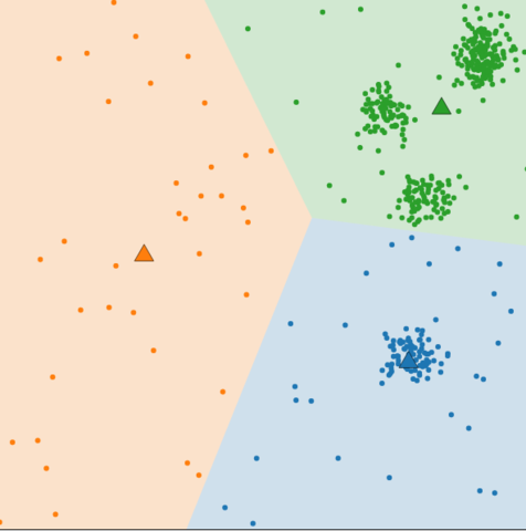
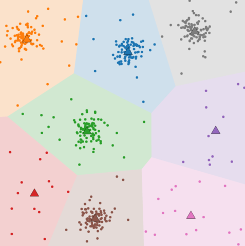
Cluster number K
- Less K
- Bigger K
-
Solution
- Find optimal K
-
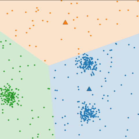
Local minimum
- Initial point
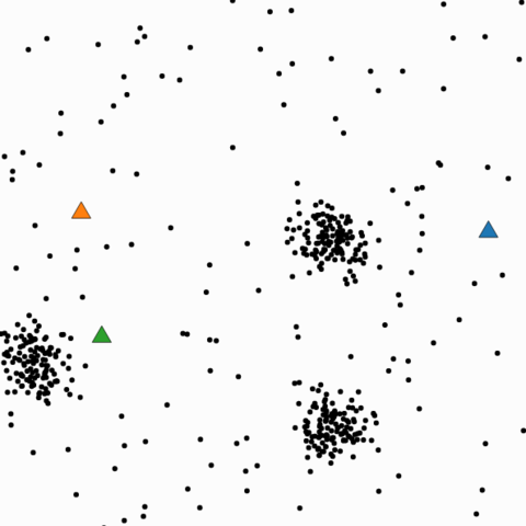
- Final result
-
Solution
- K-means ++
-
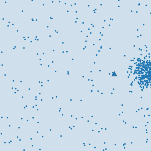
Sensitive to outliers.
- Noisy data
-
Solution
- Filtering
-
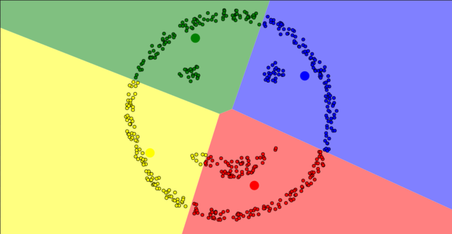
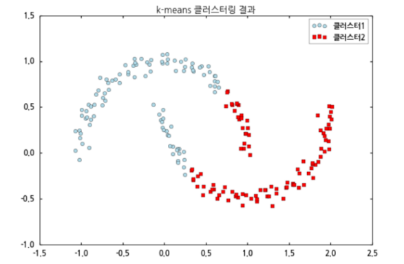
Non-spherical data
- Non-spherical data
-
Solution
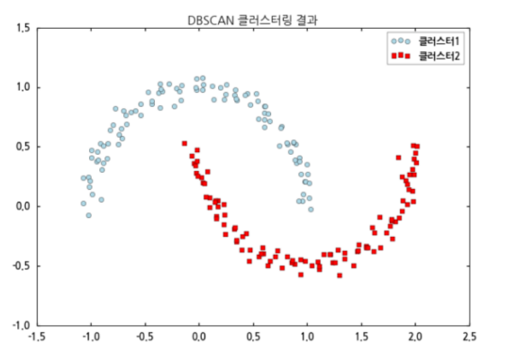
- DBSCAN
Cluster number - K decision
- Rule of thumb
-
Elbow method
-
Monitor the results while increasing the number of clusters sequentially.
-
If adding one cluster does not give a much better result than before, set the number of clusters to the number of clusters you want to find.
-
군집내 군집과 개체간 거리 제곱합의 총합 - tot.withinss: Total within-cluster sum of squares
-
-
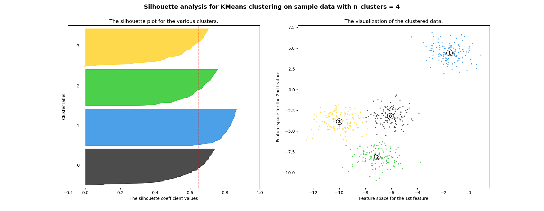
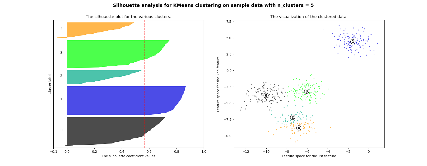
Silhouette Method [3]
-
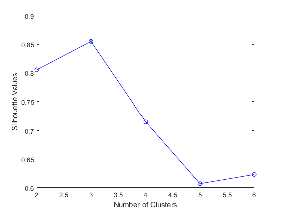
Can be used to evaluate the validity of clustering results and to select an appropriate number of clusters .
-
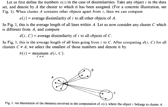
Parameters
-
비적합도 -> d(i,C) - 모든 클러스터에 대해서 계산
-
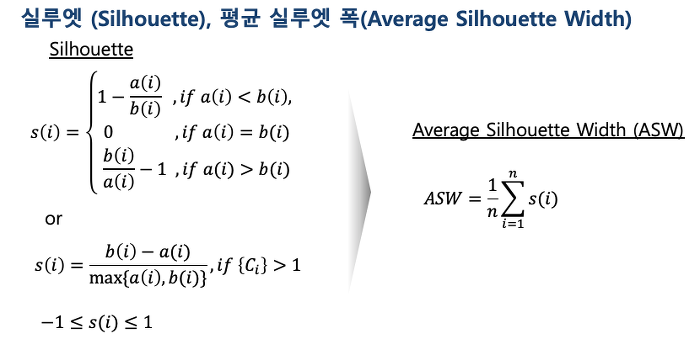
The relative quality of the clusters
-
If the silhouette value is close to 1, it means that the distance between objects in the same cluster is closer than that of other clusters, so it means that object i is well clustered
-
S(i) -> 적합도
-
a(i),b(i) 비적합도
-
If many objects have low or negative silhouette values, it can be determined that the cluster composition is too large or has too few clusters.
-
K-means++[4]
- Select first centroid from data as random
- Subsequent centroids adjust the sampling probability distribution so that points with a large distance from the previously selected centroid are selected with high probability. Pick a point based on this distribution.
-
Repeat previous step as K-1
Hierarchical clustering
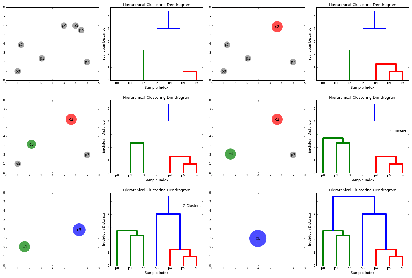
- Start clustering from a small unit and proceed with clustering in a bottom-up method that repeats until all data is bundled.
Bottom-up(Agglomerative)
- Single link

- Complete link

- Average link

- Centroid link

- Ward's method
Top-down(Division)
- DIANA method
DBSCAN[1]
- Compared to the previous clustering, it is a technique that includes the concept of density.
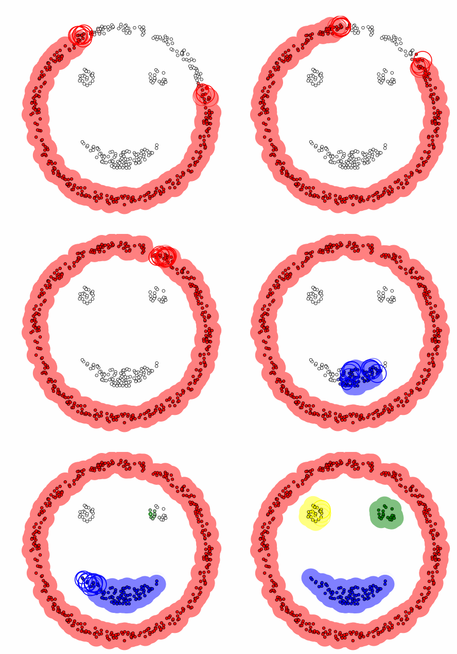
Algorithm
-
Input
- radius
- minPts
-
Select random points
-
Point decision
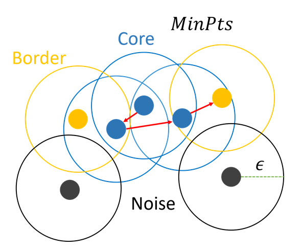
- Repeat previous step for neighbor data
Initialization method
-
There is no such thing as a formula or objective statistic to obtain the theoretically proven DBSCAN input parameters MinPts and Eps. There are only subjective heuristic methods that can help you determine MinPts and Eps.
-
MinPts
- In DBSCAN's original paper (ref [1]), recommended to set MinPts = 4 for 2D data. (Because of computation load)
- There is also a paper (ref [2]) that recommends MinPts = 2 * dim for datasets with more variables than two dimensions.
- Heuristic way to determines MinPts = ln(n) (where n as number os points in database)
-
Eps
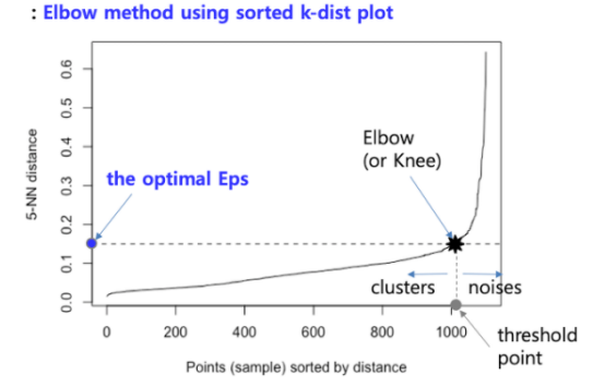
- Find the distance k-dist from one point to the k nearest points, that is, k_NN (k-Nearest Neighbor).
- Sort the k-dist in descending order, and draw the k-dist on the Y-axis by the sorted points on the X-axis.
- Using the Elbow method, the k-dist of the first "valley" point is determined as Eps.
Limitation
- DBSCAN performs many calculations and slower than k-means
- It is greatly influenced by the radius and threshold settings.
- 'Curse Of dimensionality', which is a common disadvantage of all data models using Euclidean squared distance is existence.
- It is a problem that the amount of required training data increases rapidly as the higher-dimensional dataset goes, and this has the disadvantage of requiring a lot of calculations.
- DBSCAN is not entirely deterministic. That's because the algorithm starts with a random point. Therefore border points that are reachable from more than one cluster can be part of either cluster.
Comparison
-
k-means
-
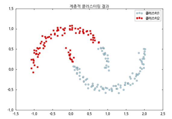
Hierarchical clustering
-
DBSCAN
- for more -> LiDAR(PCL)에 대한 사례 // MATLAB 예제 -- 예시 응용하는 위주로 // plane fitting의 경우 RANSAC, plane clustering
[Reference]
* [1] Martin Ester, Hans-Peter Kriegel, Jorg Sander, Xiaowei Xu, 1996, "A Density-Based Algorithm for Discovering Clusters in Large Spatial Databases with Noise", KDD-96
* [2] Erich Schubert, Jorg Sander, Martin Ester, Hans Peter Kriegel, Xiaowei Xu, 2017, "DBSCAN Revisited: Why and How You Should (Still) Use DBSCAN
* [3] Peter J. Rousseeuw, Journal of Computational and Applied Mathematics 20 (1987), "Silhouettes: a Graphical Aid to the Interpretation and Validation of Cluster Analysis"
* [4] Arthur, D. and Vassilvitskii, S. (2007). 〈k-means++: the advantages of careful seeding〉 (PDF). 《Proceedings of the eighteenth annual ACM-SIAM symposium on Discrete algorithms》. Society for Industrial and Applied Mathematics Philadelphia, PA, USA. 1027–1035쪽.

