[Paper Review] DeepFM

승민·2025년 10월 16일

본 글은 2017년 발표된 DeepFM: A Factorization-Machine based Neural Network for CTR Prediction을 읽고 요약 및 정리한 글입니다.
논문
직접 구현 DeepFM 모델 코드 (Pytorch)
직접 구현 DeepFM Movielens100k 학습 코드 (Jupyter)

0. Summary

Wide & Deep vs DeepFM

항목	Wide & Deep	DeepFM
구성	Wide (Linear model) + Deep(MLP)	FM (low-order interactions) + Deep(high-order interactions)
Feature Engineering	수동 Feature Cross 필요	자동 Feature Factorization Machines 학습
Embedding 공유	❌ (Wide와 Deep 입력 분리)	✅ (FM과 Deep이 Embedding Layer 공유)
Interaction Modeling	- Wide: 1차, 수동 조합 - Deep: 고차 비선형	- FM: 2차 상호작용 - Deep: 고차 비선형
모델 수식	$\hat{y} = \sigma(W_{wide}^T x + W_{deep}^T a^{(L)} + b)$	$\hat{y} = \sigma(\hat{y}_{FM} + \hat{y}_{Deep})$

DeepFM

구분	FM Component	Deep Component
역할	Low-order feature interaction	High-order feature interaction
목적	2차 상호작용(Feature pair) 자동 학습	복잡한 비선형 관계 학습
특징	- Pairwise interaction 자동 학습 - Linear model 기반	- 비선형 관계 학습 - MLP: Deep representation
모델 수식	① 1차 항: $w_0 + \sum_i w_i x_i$ ② 2차 항: $\sum^n_{i=1} \sum^n_{j=i+1} \langle v_i, v_j \rangle x_i x_j$	$a^{(l+1)} = \sigma(W^{(l)} a^{(l)} + b^{(l)})$ $\hat{y}_{deep} = \sigma(W_{out} a^{(L)} + b_{out})$

1. Introduction

CTR 예측은 추천시스템에서 정말 중요
low & high order feature interactions를 동시에 고려하는 것이 중요
- 효과적인 feature interactions를 모델링 필요
- 몇몇은 전문가의 수동으로 찾아내는 형태
- 대부분 데이터 속에 숨어 있는 형태
WideAndDeep
- 전문가의 feature engineering 필요
- wide, deep의 input이 다름
DeepFM
- feature engineering 필요 없음
- 공통 input 사용
- FM $\rightarrow$ low-order interactions
  - Pairwise feature interactions
  - Low-order
- DNN $\rightarrow$ sophisticated feature interactions
  - Multi-layered Perceptron
  - High-order

2. Our Approach

학습 데이터: $n$ 개의 인스턴스 $(\chi, y)$ 로 구성
- $\chi$ : $m$ 개의 fields를 갖는 레코드
  - $\mathbf{x} = [\mathbf{x}_{\text{field}_1}, \mathbf{x}_{\text{field}_2},..., \mathbf{x}_{\text{field}_m} ]$
  - 매우 고차원이고 희소
  - 범주형(one-hot), 연속형(전처리) 모두 포함 가능
- $y$ : 레이블(ex. click, acquisition)
  - $y \in \{0, 1\}$

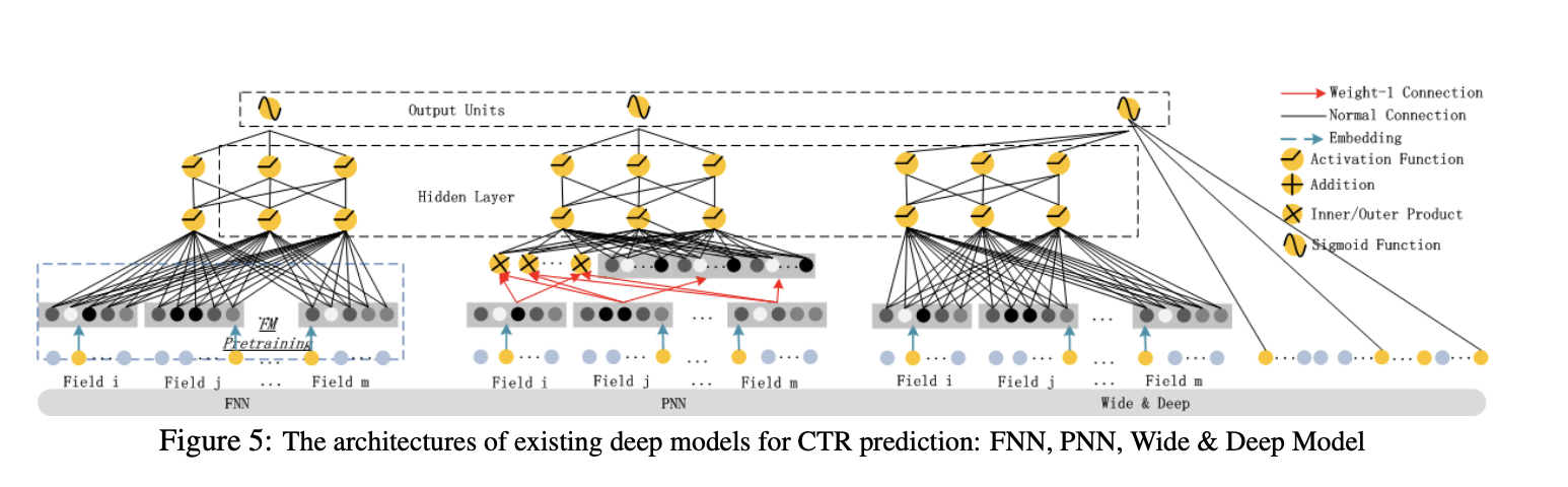
2.1 DeepFM

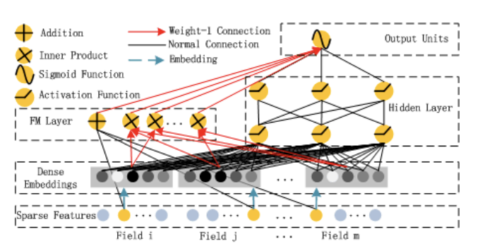
Normal Connection

Red arrow: weight1의 연결

Blue arrow: Embedding

Addion: 모든 input을 함께 더함

Wide 와 Deep Component는 동일한 raw feature vector를 공유

low- & high-order feature interactions를 함께 학습
$\hat{y} = sigmoid(y_{FM} + y_{DNN})$

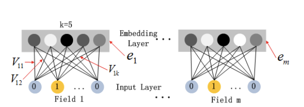
Embeddings(Input)

$w_i$ : order-1 importance

$V_i$ : 다른 피처와의 interactions 효과를 측정하는데 사용

FM component의 input으로 사용되어 order-2 feature interaction

Deep component의 input으로 사용되어 high-rder feagture interaction

FM Component

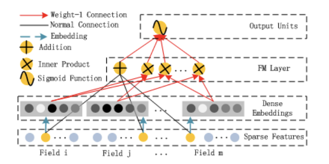
Factorization Machine

(order-1) Addition unit

(order-2) Pairwise feature interation

각각의 feature latent vector를 inner product

전혀 등장하지 않거나 거의 등장하지 않은 학습 데이터에 대해서도 학습 가능

$y_{FM} = \langle w, x \rangle + \sum^d_{j_1=1}\sum^d_{j_2=j_1+1} \langle V_i, V_j \rangle x_{j_1} \cdot x_{j_2}$

Deep Component

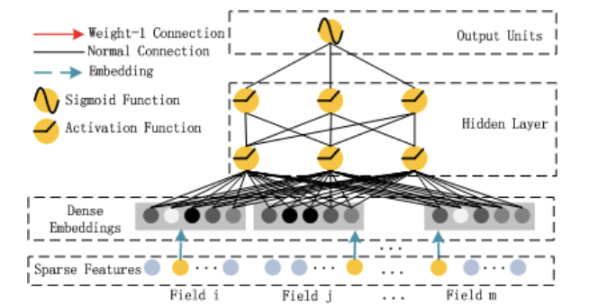
DNN
high-order feature interactions
- image, audio 등과 달리 추천에서는 high-sparse feature가 만흥ㅁ
- dense embedding 후 사용(embedding layer)

2.2 Relationship with the other Neural Network

다른 Network와 비교

	No Pre-training	High-order Features	Low-order Features	No Feature Engineering
FNN	×	√	×	√
PNN	√	√	×	√
Wide & Deep	√	√	√	×
DeepFM	√	√	√	√

3. Experiment Setup

3.1 Experiment Setup

Dataset
- Criteo
  - 45 million users click records
  - 13 continuous features
  - 26 categorical features
  - split dataset randomly
    - train: 90%
    - test: 10%
- Company
  - 1billion records
  - app features(identification, category, ...)
  - user feature4s(user's downloaded apps, ...)
  - context features(time, ....)
    - train: 연속 7일 동안 app store의 game center 클릭 기록
    - test: 다음 하루

3.2 Performance Evaluation

Efficiency
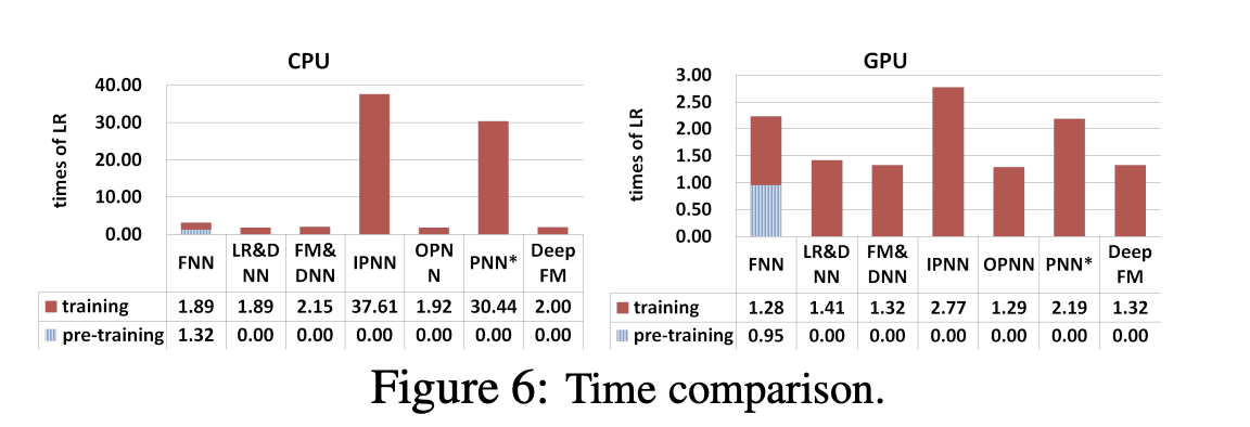
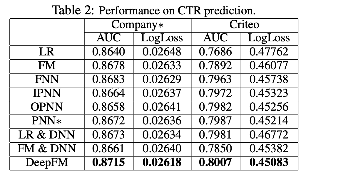
$\frac{\text{training time of deep CTR model}}{\text{training time of LR}}$
Effectiveness
- LR: feature interactions를 학습하는게 성능에 기여
- high- and low-order feature interactions 학습하는게 성능에 기여
  - FM: low-order
  - FNN, IPNN, OPNN, PNN: high-order
- embedidng을 공유하여 high- and low-order feature interactions을 동시에 학습
  - LR & DNN, FM & DNN: separate feature embedding