데이터 주도 학습과 신경망 학습

1. 데이터 주도 학습

• 데이터 주도 학습은 신경망이 데이터를 보고 스스로 최적의 가중치와 편향을 찾아가는 과정
• 사람이 직접 설정 안 하고, 데이터로 자동 학습

핵심 포인트

• 가중치 매개변수: 신경망이 입력을 출력으로 바꿀 때 쓰는 값들. 이걸 조정해서 예측을 더 정확하게 만듦.
• 데이터로 학습: 데이터를 보고 가중치를 자동으로 조정해서 모델이 똑똑해지게 하는 것

훈련 데이터랑 테스트 데이터

신경망 학습에 쓰는 데이터는 두 종류:
1. 훈련 데이터: 모델이 학습할 때 쓰는 데이터. 가중치 조정에 사용.
2. 테스트 데이터: 학습 끝난 모델의 성능을 확인하는 데이터. 훈련에 안 썼던 별도의 데이터로, 모델이 새 데이터에서도 잘 작동하는지 봄.

왜 데이터를 나눠?

• 범용성: 훈련 데이터만 쓰면 모델이 그 데이터에만 너무 잘 맞춰질 수 있음(오버피팅). 테스트 데이터로 새 데이터에서도 잘 작동하는지 확인.
• 예: MNIST 손글씨 숫자 데이터셋에서 60,000장은 훈련, 10,000장은 테스트로 씀.

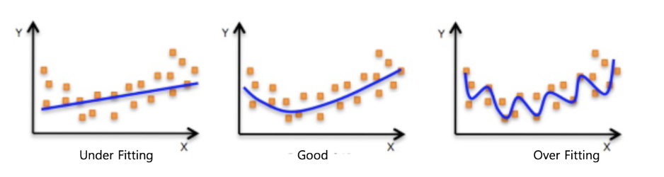
오버피팅

• 정의: 모델이 훈련 데이터에 너무 최적화돼서 새 데이터(테스트 데이터)에서 성능이 떨어지는 것.
• 예: 학생이 시험 문제만 외워서 그 문제는 잘 풀지만 비슷한 새 문제는 못 푸는 거랑 비슷.
• 해결법: 훈련/테스트 데이터 분리, 모델 복잡도 조정, 정규화 기법 사용.

---

2. 손실 함수(Loss Function)

• 모델 예측이 얼마나 틀렸는지 숫자로 보여주는 함수
• 신경망은 이 손실 값을 최소화하도록 가중치를 조정함

손실 함수의 역할

• 지표: 모델 성능을 숫자로 표현.
• 최적화 방향: 손실 값을 줄이는 방향으로 가중치 조정.
• 예: 예측이 실제값에 가까울수록 손실 값이 작아짐.

주요 손실 함수

1. 평균 제곱 오차 (Mean Squared Error, MSE)

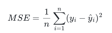
• 정의: 예측값과 실제값 차이를 제곱한 뒤 평균 내는 거.
• 특징: 차이가 크면 손실 값이 급격히 커짐. 연속적인 값 예측할 때 주로 사용.
• 수식:
  $\text{MSE} = \frac{1}{2} \sum (y - t)^2$
  여기서 $y$는 예측값, $t$는는 실제값.

코드

import numpy as np

def mean_squared_error(y, t):
    return 0.5 * np.sum((y - t)**2)

• 코드 설명:
  • y: 모델 예측값 (예: [0.6, 0.3, 0.1]).
  • t: 실제값 (예: [1, 0, 0]).
  • (y - t)**2: 차이를 제곱.
  • np.sum: 차이 제곱의 합.
  • 0.5: 수치 안정성 위해 곱함.
• 결과: MSE 값 작을수록 예측이 실제값에 가까움.

예시

y = np.array([0.6, 0.3, 0.1])  # 예측값
t = np.array([1, 0, 0])        # 실제값
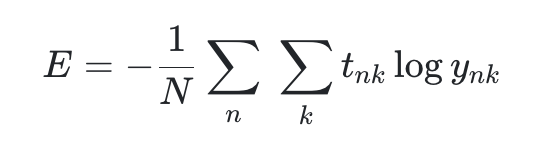
print(mean_squared_error(y, t))  # 출력: 0.125

2. 교차 엔트로피 오차 (Cross Entropy Error, CEE)

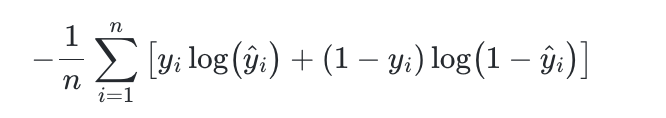
• 정의: 예측 확률과 실제 레이블 간 차이를 측정. 분류 문제에 주로 사용.
• 특징: 예측이 실제값에 가까울수록 손실 값 작아짐. 이진/다중 클래스 분류에 적합.
• 수식:
  $\text{CEE} = -\sum t \cdot \log(y)$
  여기서 $y$는 예측 확률, $t$는 실제 레이블(보통 one-hot encoding).

코드

def cross_entropy_error(y, t):
    delta = 0.0000001  # log(0) 방지용
    return -np.sum(t * np.log(y + delta))

• 코드 설명:
  • y: 예측 확률 (예: [0.6, 0.3, 0.1]).
  • t: 실제 레이블 (예: [0, 0, 1]).
  • np.log(y + delta): 예측값에 로그 취해서 확률 차이 계산. delta는 0 로그 방지.
  • -np.sum(t * ...): 실제값과 로그 곱한 뒤 합산.
• 결과: CEE 값 낮으면 예측 정확, 높으면 틀린 거.

예시

y = np.array([0.6, 0.3, 0.1])  # 예측 확률
t = np.array([0, 0, 1])        # 실제 레이블
print(cross_entropy_error(y, t))  # 출력: 약 2.302585

---

3. 미니배치 학습

• 훈련 데이터 일부만 써서 손실 함수 계산하고 가중치 갱신하는 방법
• 모든 데이터를 한꺼번에 쓰는 배치 학습보다 효율적

왜 미니배치?

• 효율성: 데이터 전부 처리하면 계산량 많음. 미니배치는 일부만 써서 빠름.
• 일반화: 무작위로 뽑은 데이터로 학습하니까 특정 데이터에 치우치지 않음.
• 예: MNIST 데이터 60,000장 중 100장 무작위로 뽑아서 학습.

코드

from mnist import load_mnist
import numpy as np

(X_train, t_train), (X_test, t_test) = load_mnist(normalize=True, one_hot_label=True)

train_size = X_train.shape[0]  # 60,000
batch_size = 10
batch_mask = np.random.choice(train_size, batch_size)  # 10개 무작위 선택

x_batch = X_train[batch_mask]  # 선택된 데이터
t_batch = t_train[batch_mask]  # 선택된 레이블

• 코드 설명:
  • load_mnist: MNIST 데이터 불러옴. normalize=True로 0~1 정규화, one_hot_label=True로 레이블 one-hot encoding.
  • np.random.choice: 60,000개 중 10개 무작위 선택.
  • x_batch, t_batch: 선택된 데이터와 레이블로 미니배치 구성.

미니배치용 CEE

미니배치에서는 여러 샘플 손실 값을 평균냄.

def cross_entropy_error(y, t):
    if y.ndim == 1:  # 1차원 입력 처리
        t = t.reshape(1, t.size)
        y = y.reshape(1, y.size)
    
    batch_size = y.shape[0]
    return -np.sum(t * np.log(y)) / batch_size

• 코드 설명:
  • y.ndim == 1: 단일 샘플 입력이면 2차원으로 변환.
  • batch_size: 미니배치 크기.
  • / batch_size: 손실 값 평균 내서 배치 크기에 상관없이 일정.

---

4. 미분과 신경망 학습

• 미분은 손실 함수 기울기 계산해서 가중치 갱신에 쓰임
• 기울기는 손실 값이 작아지는 방향을 알려줌

미분의 역할

• 가중치 갱신: 손실 함수를 가중치로 미분해 기울기 구하고, 그 방향으로 가중치 조정.
• 연속적 변화: 손실 함수는 가중치 변화에 따라 부드럽게 변해서 미분 가능.
• 대조: 정확도는 불연속적이어서 미분 안 됨. 그래서 손실 함수 씀.

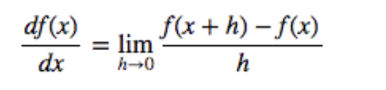
수치 미분 (Numerical Differentiation)

• 작은 변화량으로 기울기 근사하는 방법.
  

코드

def numerical_diff(f, x):
    h = 0.0001
    return (f(x + h) - f(x)) / h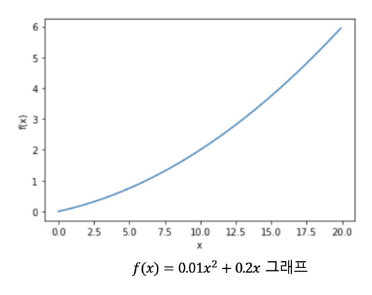

• 코드 설명:
  • f: 미분할 함수.
  • x: 미분 지점.
  • h: 작은 값(0.0001)으로 변화량 계산.
  • (f(x + h) - f(x)) / h: 함수 변화량 나누기로 기울기 구함.

예시 함수

def function_1(x):
    return 0.01 * x**2 + 0.1 * x

• 함수 설명: $f(x) = 0.01x^2 + 0.1x$, 2차 함수로 기울기 계산해 최솟값 찾음.

미분 계산

print(numerical_diff(function_1, 5))   # 출력: 약 0.2
print(numerical_diff(function_1, 10))  # 출력: 약 0.3

• 결과 설명:
  • $x = 5$: 기울기는 약 $0.2$
  • $x = 10$: 기울기는 약 $0.3$
  • $x$가 커질수록 기울기가 증가함

편미분 (Partial Differentiation)

• 다변수 함수에서 한 변수만 미분하는 거. 다른 변수는 고정.

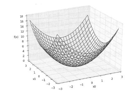
예시 함수

def function_2(x):
    return x[0]**2 + x[1]**2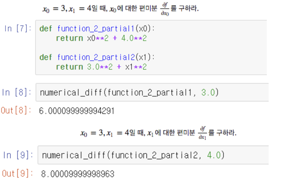

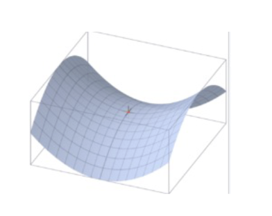
• 함수 설명: $f(x_0, x_1) = x_0^2 + x_1^2$, 2차원 2차 함수. 원점(0, 0)에서 최솟값.

---

5. 기울기와 경사하강법

기울기 (Gradient)

• 손실 함수가 작아지는 방향을 나타냄
• 다변수 함수에서는 각 변수의 편미분을 벡터로 모음

코드

def numerical_gradient(f, x):
    h = 0.0001
    grad = np.zeros_like(x)
    
    for index in range(x.size):
        tmp_val = x[index]
        x[index] = tmp_val + h
        fxh1 = f(x)
        
        x[index] = tmp_val
        fxh2 = f(x)
        
        grad[index] = (fxh1 - fxh2) / h
    
    return np.round(grad, 3)

• 코드 설명:
  • np.zeros_like(x): $$ x $$와 같은 크기의 0 벡터.
  • 각 변수에 수치 미분 계산해 기울기 벡터 채움.
  • np.round(grad, 3): 소수점 3자리로 반올림.

예시

x = np.array([3.0, 4.0])
print(numerical_gradient(function_2, x))  # 출력: [6. 8.]
x = np.array([0.0, 2.0])
print(numerical_gradient(function_2, x))  # 출력: [0. 4.]

• 결과 설명:

  • $x = [3, 4]$: 기울기 $\nabla f = [6, 8]$
    → $x_0$ 방향으로 6, $x_1$ 방향으로 8 증가

  • $x = [0, 2]$: 기울기 $\nabla f = [0, 4]$
    → $x_0$는 최솟값 근처라 0, $x_1$ 방향만 변화

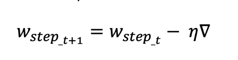
경사하강법 (Gradient Descent)

• 기울기 써서 손실 함수 최솟값 찾는 방법
• 기울기 방향으로 가중치 갱신

코드

def gradient_descent(f, init_x, lr=0.01, step_num=100):
    x = init_x
    x_history = []
    
    for i in range(step_num):
        x_history.append(x.copy())
        grad = numerical_gradient(f, x)
        x -= lr * grad  # 기울기 반대 방향 이동
    
    return x, np.array(x_history)

• 코드 설명:
  • f: 최적화할 함수.
  • init_x: 초기 가중치.
  • lr: 학습률 (한 번에 얼마나 이동).
  • step_num: 반복 횟수.
  • x -= lr * grad: 기울기 반대 방향으로 갱신.

예시

init_x = np.array([-3.0, 4.0])
lr = 0.1
step_num = 100

x, x_history = gradient_descent(function_2, init_x, lr, step_num)
print(x)  # 출력: [-0.0002, 0.0001]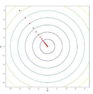

• 결과 설명:
  • 초기값 $[-3, 4]$에서 시작해 100번 반복 후 $[0, 0]$ 근처로 수렴함
  • 함수 $f(x_0, x_1) = x_0^2 + x_1^2$의 최솟값은 원점인 $(0, 0)$

---

6. 옵티마이저 (Optimizer) 자세히 알아보기

• 손실 함수 최소화하도록 가중치 갱신하는 알고리즘.
• 경사하강법을 개선한 여러 방법이 있음.

1. 확률적 경사하강법 (Stochastic Gradient Descent, SGD)

• 정의: 무작위로 뽑은 데이터(미니배치)로 기울기 계산해 가중치 갱신.
• 특징:
  • 매번 랜덤 데이터 써서 국소 최적해에 빠질 가능성 줄임.
  • 계산 빠름.
• 단점: 기울기 0인 지점에서 멈출 수 있음. 학습이 불안정할 때도 있음.
• 예: MNIST 데이터 100장 무작위로 뽑아서 기울기 계산.

코드 (간단한 SGD)

def sgd_update(params, grad, lr=0.01):
    params -= lr * grad
    return params

• 설명: params는 가중치, grad는 기울기, lr은 학습률. 기울기 반대 방향으로 갱신.

2. 모멘텀 (Momentum)

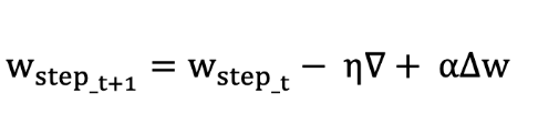
• 정의: 이전 기울기를 고려해 관성 추가. 공이 언덕 굴러가는 것처럼 동작.
• 특징:
  • 속도 벡터 유지해서 국소 최적해 탈출 쉬움.
  • 학습이 더 부드럽게 진행.
• 수식:

• $v$: 속도
• $\alpha$: 모멘텀 계수 (보통 0.9)
• $\eta$: 학습률
• $\nabla L$: 손실 함수의 기울기

• 예: 언덕에서 공이 굴러가다 작은 구덩이 넘어서 계속 내려가는 느낌.

코드 (간단한 모멘텀)

def momentum_update(params, grad, velocity, lr=0.01, momentum=0.9):
    velocity = momentum * velocity - lr * grad
    params += velocity
    return params, velocity

• 설명: velocity로 이전 기울기 정보 유지. 새 기울기와 결합해 갱신.

3. 아다그라드 (AdaGrad)

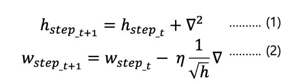
• 정의: 가중치별로 학습률 자동 조정. 많이 이동한 가중치는 학습률 줄임.
• 특징:
  • 초기 학습 빠르고, 자주 업데이트된 가중치는 천천히 움직임.
  • ( h )라는 변수로 과거 기울기 제곱 합 저장.
• 수식:
  $h \leftarrow h + (\nabla L)^2$

• $h$: 과거 제곱 기울기의 누적합
• $\epsilon$: 0 나눗셈 방지를 위한 작은 값

• 단점: 학습 오래되면 ( h ) 커져서 학습률 너무 작아질 수 있음.

코드 (간단한 AdaGrad)

def adagrad_update(params, grad, h, lr=0.01, epsilon=1e-8):
    h += grad ** 2
    params -= lr * grad / (np.sqrt(h) + epsilon)
    return params, h

• 설명: h로 기울기 제곱 합 누적. 학습률을 $\sqrt{h}$로 나눠 조정.

4. RMSProp

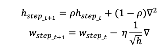
• 정의: AdaGrad의 학습률 감소 문제 개선. 최근 기울기만 고려.
• 특징:
  • ( h ) 계산 시 지수 이동 평균 써서 오래된 기울기 영향 줄임.
  • 안정적이고 빠른 수렴.
• 수식:
  $h \leftarrow \rho h + (1 - \rho)(\nabla L)^2$

• $\rho$: 지수 이동 평균 비율 (보통 0.9)

코드 (간단한 RMSProp)

def rmsprop_update(params, grad, h, lr=0.01, rho=0.9, epsilon=1e-8):
    h = rho * h + (1 - rho) * (grad ** 2)
    params -= lr * grad / (np.sqrt(h) + epsilon)
    return params, h

• 설명: rho로 최근 기울기 강조. ( h )가 너무 커지지 않음.

5. 아담 (Adam)

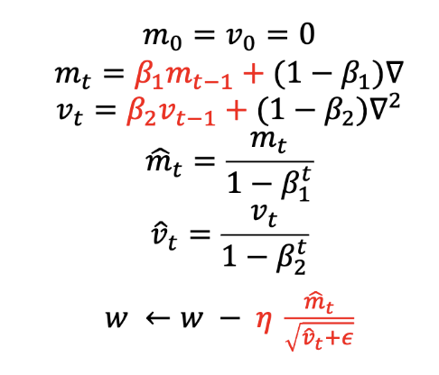
• 정의: 모멘텀과 RMSProp 결합. 가장 인기 있는 옵티마이저.
• 특징:
  • 모멘텀으로 속도 유지, RMSProp으로 학습률 조정.
  • 빠르고 안정적으로 최솟값 찾음.
• 수식:
  $m \leftarrow \beta_1 m + (1 - \beta_1)\nabla L$

• $m$: 1차 모멘텀 추정치 (기울기의 평균)
• $v$: 2차 모멘텀 추정치 (기울기의 제곱 평균)
• $\beta_1 \approx 0.9$, $\beta_2 \approx 0.999$

코드 (간단한 Adam)

def adam_update(params, grad, m, v, t, lr=0.001, beta1=0.9, beta2=0.999, epsilon=1e-8):
    t += 1
    m = beta1 * m + (1 - beta1) * grad
    v = beta2 * v + (1 - beta2) * (grad ** 2)
    m_hat = m / (1 - beta1 ** t)
    v_hat = v / (1 - beta2 ** t)
    params -= lr * m_hat / (np.sqrt(v_hat) + epsilon)
    return params, m, v, t

• 설명: m으로 모멘텀, v로 학습률 조정. t로 바이어스 보정.

어떤 옵티마이저 써야 해?

• SGD: 간단하고 이해 쉬움. 튜닝 필요.
• 모멘텀: 국소 최적해 탈출 좋아. SGD보다 부드러움.
• AdaGrad: 초기 학습 빠름. 깊은 학습에선 멈출 수 있음.
• RMSProp: AdaGrad 개선. 안정적.
• Adam: 대부분 상황에서 잘 작동. 기본 선택으로 추천

---

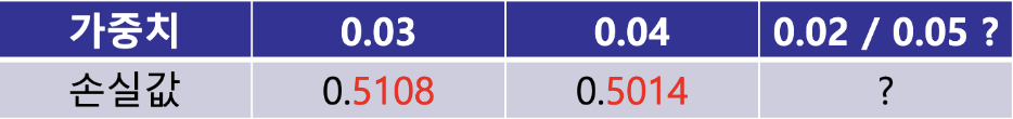
7. 학습률 (Learning Rate)

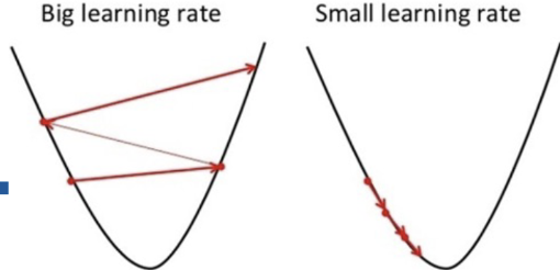
• 가중치가 기울기 방향으로 얼마나 이동할지 정함

• 큰 학습률: 빠르게 학습. 근데 최솟값 지나칠 수 있음.

• 작은 학습률: 안정적. 근데 너무 느림.

• 예: 학습률 0.01은 천천히, 0.1은 빠르게.

---

8. 배치 크기 (Batch Size)

• 한 번에 처리하는 데이터 양
• 배치 크기에 따라 학습 방식 달라짐

1. 온라인 학습

• 특징: 데이터 1개씩 처리.
• 장점: 갱신 빠름.
• 단점: 잘못된 방향으로 갈 수 있음.

2. 배치 학습

• 특징: 모든 데이터 처리 후 평균 손실로 갱신.
• 장점: 안정적.
• 단점: 계산량 많음.

3. 미니배치 학습

• 특징: 일부 데이터(예: 100개) 무작위로 뽑아서 처리.
• 장점: 효율적이고 안정적.
• 예: MNIST 60,000장 중 100장 선택.

---

9. 신경망 학습 절차

신경망 학습은 4단계로 진행:
1. 미니배치: 훈련 데이터 일부 무작위로 뽑음.
2. 기울기 계산: 뽑은 데이터로 손실 함수 기울기 구함.
3. 가중치 갱신: 기울기 방향으로 가중치 조금 갱신.
4. 반복: 1~3 반복해서 손실 값 줄임.

---

10. 실제 신경망 구현

간단한 신경망 클래스

class simpleNet:
    def __init__(self):
        self.W = np.random.randn(2, 3)  # 2x3 가중치 초기화
    
    def predict(self, x):
        return np.dot(x, self.W)  # 입력과 가중치 행렬곱
    
    def loss(self, x, t):
        z = self.predict(x)
        y = softmax(z)  # 소프트맥스로 확률
        loss = cross_entropy_error(y, t)  # 손실 계산
        return loss

• 설명:
  • self.W: 2x3 랜덤 가중치.
  • predict: 입력 ( x )와 가중치 ( W ) 행렬곱으로 예측.
  • loss: 예측값 소프트맥스로 변환 후 CEE로 손실 계산.

소프트맥스 함수

def softmax(a):
    exp_a = np.exp(a)
    sum_exp_a = np.sum(exp_a)
    y = exp_a / sum_exp_a
    return y

• 설명: 입력을 확률로 변환. 출력 합이 1.

사용 예시

net = simpleNet()
x = np.array([0.6, 0.9])  # 입력
p = net.predict(x)  # 예측
print(np.argmax(p))  # 출력: 2 (최고 확률 클래스)
t = np.array([0, 0, 1])  # 정답 레이블
print(net.loss(x, t))  # 출력: 약 0.465544

가중치 미분

def f(W):
    return net.loss(x, t)

dW = numerical_gradient(f, net.W)  # 출력: [[-0.541 0.164 0.377], [-0.811 0.246 0.565]]

• 설명: 손실 함수를 가중치로 미분해 기울기 구함.