💡Neural Network

A machine learning model that mimics the way the human brain processes information

---

🎨 Batch

A method of dividing the entire dataset into several small groups to solve memory and computation speed issues during dataset training

Emergence of Batch

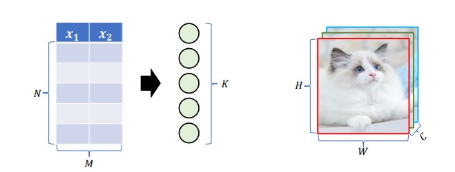
• Structure of Neural Network
  • Neural networks consist of an input layer that receives data, hidden layers that compute the input data, and an output layer that makes predictions based on the computed results
  • If the data entering the input layer is in $N X M$ format, the hidden layer corresponding to the first layer must be in $M X K$ format (where K is the number of neurons)
  • Note that image data is 3-dimensional data (height, width, channel), so the first hidden layer must be designated in a 3-dimensional format
    

Understanding Batch

• Passing data through the neural network one by one tens of thousands of times can take an immense amount of time
• Therefore, a method of grouping data together and passing them through all at once is used; this group of data is called a Batch
• However, if too much data is grouped and passed through the neural network, it becomes heavy, so we break the data into smaller portions and pass them, which is called Mini Batch
• Key Concepts
  • Batch Size: The number of data samples processed by the model in one learning step
    • For example, if there are 10,000 samples in the dataset and the Batch Size is 32, 32 samples are used in one training step
    • This process of the model learning through several batches of the dataset is repeated
  • Epoch: The process of passing the entire dataset through the model once
    • For example, if the dataset is divided into 1,000 batches, completing 1 epoch means all 1,000 batches have been used
  • Iteration: The process of processing one batch
    • For example, if the Batch Size is 32 and the dataset has 1,000 samples, you need to train 31 times with 32 samples to process the entire dataset once -> These 31 processes are each called an iteration
• Stages of Batch Training
  1. Forward Propagation: Input a batch of data into the model to compute predictions -> Each data point is processed by the model’s parameters (weights, biases) to make predictions
  2. Loss Calculation: Compare the predicted values with the actual values and calculate the error through the Loss Function
  3. Backpropagation: Calculate gradients for each parameter based on the loss value
     • Gradients represent how much each parameter affects the loss
     • The backpropagation algorithm is used to calculate gradients for each parameter and optimize them
  4. Weight Update: Use an optimization algorithm (e.g., SGD or Adam) to update the parameters
  5. Iteration: After completing the above steps for one batch, process the next batch -> This process is repeated for the entire dataset several times for learning
• Types of Batch Processing
  • SGD (Stochastic Gradient Descent): Sets the batch size to 1, processes one sample at a time, and updates the weights for each sample
    • Uses less memory and computes faster, but may have slower convergence due to noise generated by processing each sample
  • Mini-Batch Gradient Descent: The most commonly used method, processes the data in smaller batches
    • Batch sizes are typically set to values like 16, 32, 64, or 128
    • Balances between the instability of SGD and memory efficiency, achieving a good balance of training speed and stability
  • Batch Gradient Descent: Processes the entire dataset in one go
    • Has very high memory usage and may take a long time to process, but its convergence is stable
    • May not be practical for large datasets due to memory limitations

🎨 Cross-Entropy Error

A Loss Function used to measure the difference between the predicted probability distribution and the actual target distribution, evaluating how close the predicted values are to the actual values.

Cross Entropy

• Definition: A function that measures the difference between two probability distributions

  • Mainly used to evaluate how closely the predicted distribution matches the actual distribution in classification problems.
  • Here, "probability distribution" refers to the probability that the predicted value belongs to each class, and Cross Entropy numerically evaluates how accurate that prediction is.
  • The further the prediction is from the actual value, the larger the Cross Entropy value becomes -> This is designed to give large penalties for incorrect predictions.

• Formula

  • General Cross Entropy Formula
    • It calculates the difference between the true distribution $P$ and the predicted distribution $Q$ by taking the logarithm, numerically quantifying the error for each prediction.
  $H(P,Q) = -\sum_x P(x)\log Q(x)$

  • $P(x)$: True probability distribution of the data

  • $Q(x)$: Predicted probability distribution of the model

  • $x$: The set of all possible outcomes

  • Binary Cross Entropy: Assigns large penalties for incorrect predictions, guiding the model towards correct predictions.

    • When $y_i$ is 1, meaning the class is correct, $\log(\hat{y}_i)$ is emphasized. The closer $\hat{y}_i$ is to 1, the smaller the loss.
    • When $y_i$ is 0, the term $(1 - \hat{y}_i)$ becomes important. The closer the prediction is to 0, the smaller the loss.
    $L = -\frac{1}{n}\sum_{i=1}^n (y_i \log(\hat{y_i}) + (1-y_i)\log(1-\hat{y_i}))$
    • $y_i$: Actual label (0 or 1)
    • $\hat{y}_i$: Predicted probability (value between 0 and 1)

  • Categorical Cross Entropy: Imposes a large penalty when the model fails to predict the correct class with high probability.

    • The logarithm of the predicted probability for the actual class is used for each data point -> The larger the predicted probability for the actual class, the smaller the loss.
    $L = - \sum_{i=1}^n \sum_{k=1}^K y_{i,k} \log(\hat{y}_{i,k})$
    • $K$: Number of classes
    • $y_{i,k}$: Actual class (1 if the class is correct, otherwise 0)
    • $\hat{y}_{i,k}$: Predicted probability for class $k$

Relationship with Softmax Function

• The Softmax function converts the logits predicted by the model into probabilities, allowing Cross Entropy to evaluate the probabilities for each class.

  $\hat{y}_k = \frac{e^{z_k}}{\sum_{j=1}^K e^{z_j}}$
  • $z_k$: Logit for class $k$ (model output value)

• The Softmax function calculates the probabilities for each class and normalizes them so that the sum of all class probabilities equals 1.

• Cross Entropy then calculates the difference between these probabilities and the actual labels.

Example Usage of Cross Entropy

• Problem Setup

  • Assume the model is classifying among three classes. For example, the classes are:
    • Class 1: Cat
    • Class 2: Dog
    • Class 3: Elephant
  • Assume the logits predicted by the model are:
    • Logit values: $z_1 = 2.0$, $z_2 = 1.0$, $z_3 = 0.1$
  • The actual label is Class 1 (Cat), and in one-hot encoding:
    $y = [1,0,0]$

• Softmax Function Calculation

  • Calculate the probability for each class:

    $\hat{y}_1 = \frac{e^{2.0}}{e^{2.0} + e^{1.0} + e^{0.1}} = \frac{7.389}{7.389 + 2.718 + 1.105} = \frac{7.389}{11.212} \approx 0.659$
    $\hat{y}_2 = \frac{e^{1.0}}{e^{2.0} + e^{1.0} + e^{0.1}} = \frac{2.718}{11.212} \approx 0.242$
    $\hat{y}_3 = \frac{e^{0.1}}{e^{2.0} + e^{1.0} + e^{0.1}} = \frac{1.105}{11.212} \approx 0.099$

  • Predicted probabilities:

    $\hat{y} = [0.659, 0.242, 0.099]$

• Cross Entropy Loss Calculation

  • Given the actual label $y = [1, 0, 0]$ and the predicted probabilities $\hat{y} = [0.659, 0.242, 0.099]$:

    $L = -(1 \cdot \log(0.659) + 0 \cdot \log(0.242) + 0 \cdot \log(0.099))$

  • Thus,

    $L = -\log(0.659) \approx -(-0.417) = 0.417$

  • Therefore, the Cross Entropy Loss is 0.417.