Backward propagation

💡 Backward propagation

Algorithm based on the chain rule

---

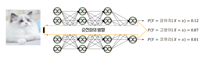
🥨 Forward Propagation

Data is propagated from the input layer to the output layer, with calculations occurring at each neuron.

1. Transmission of input data: The input data $\mathbf{X}$ is passed to the input layer of the neural network, typically in the following form:

   $\mathbf{X} = {[x_1, x_2, x_3, ..., x_n]}^T$
   • Here, $n$ is the number of input features.

2. Linear Transformation: The neurons in each layer perform a linear transformation by receiving the output of the previous layer. This transformation is calculated by taking the dot product of the weights with the input and adding the bias:

   • In the first hidden layer, $\mathbf{A}^{[0]} = \mathbf{X}$
   $\mathbf{Z}^{[l]} = \mathbf{W}^{[l]} \mathbf{A}^{[l-1]} + \mathbf{b}^{[l]}$
   • $\mathbf{Z}^{[l]}$: Linear transformation result (pre-activation value) of the $l$-th layer.
   • $\mathbf{W}^{[l]}$: Weight matrix of the $l$-th layer.
   • $\mathbf{A}^{[l-1]}$: Activation (output) of the previous layer.
   • $\mathbf{b}^{[l]}$: Bias vector of the $l$-th layer.

3. Application of Activation Function: An activation function $\sigma$ is applied to the result of the linear transformation, adding non-linearity and generating the output to be passed to the next layer.

   $\mathbf{A}^{[l]} = \sigma(\mathbf{Z}^{[l]})$

4. Prediction Calculation at Output Layer: In the output layer, a suitable activation function is chosen based on the problem type to generate the final predicted values.

   • Regression problem: Linear output or identity function is used without an activation function.
   • Binary classification problem: Sigmoid function is used to convert the output to probability values.
   • Multiclass classification problem: Softmax function is used.

5. Loss Function Calculation: The predicted value $\hat{\mathbf{Y}}$ is compared with the actual value $\mathbf{Y}$.

   • For regression problems: MSE (Mean Squared Error).
   • For binary classification problems: Cross-Entropy Loss.
   • For multiclass classification problems: Multiclass Cross-Entropy Loss.

🥨 Chain Rule

• Definition: A method to calculate the derivative of a composite function.

  • Assume function $y$ is a function of the variable $u$, and $u$ is a function of the variable $x$:

    $y = f(u), u = g(x)$

  • Here, $y$ is a composite function of $x$: $y=f(g(x))$. According to the chain rule, the derivative of $y$ with respect to $x$ is expressed as:

    $\frac{dy}{dx} = \frac{dy}{du} \cdot \frac{du}{dx}$

  • In other words, the derivative of the composite function is the product of the derivative of $y$ with respect to the intermediate variable $u$ and the derivative of $u$ with respect to $x$.

• Chain Rule with Multiple Variables

  • Assume $y = f(u, v)$ is a function of two variables $u$ and $v$, and $u$ and $v$ are functions of $x$:

    $y = f(u(x), v(x))$

  • In this case, the chain rule states that the derivative of $y$ with respect to $x$ is:

    $\frac{dy}{dx} = \frac{\partial y}{\partial u} \cdot \frac{du}{dx} + \frac{\partial y}{\partial v} \cdot \frac{dv}{dx}$

  • This means that the total derivative is found by summing the products of the partial derivatives of $y$ with respect to each variable and the derivative of each variable with respect to $x$.

🥨 Backward propagation

• Definition

  • The process of calculating the gradients of each weight by propagating the error from the output layer back through the hidden layers to the input layer.
  • Chain rule is used to compute the gradients at each layer.

• Applying Chain Rule in a Single Layer

  • In a multilayer perceptron, the linear transformation in the $l$-th layer is defined as:

    $\mathbf{Z}^{[l]} = \mathbf{W}^{[l]} \mathbf{A}^{[l-1]} + \mathbf{b}^{[l]}$
    • $\mathbf{A}^{[l-1]}$: Output (activation) of the previous layer
    • $\mathbf{W}^{[l]}$: Weight matrix of the $l$-th layer
    • $\mathbf{b}^{[l]}$: Bias vector of the $l$-th layer

  • The activation value $\mathbf{A}^{[l]}$ of the $l$-th layer is calculated using the activation function $\sigma$:

    $\mathbf{A}^{[l]} = \sigma (\mathbf{Z}^{[l]})$
    • Loss function $L$: The difference between the predicted value $\hat{\mathbf{Y}}$ and the actual value $\mathbf{Y}$ from the output layer.

  • Backpropagation involves calculating the gradient $\frac{\partial L}{\partial w^{[l]}}$ of each weight $w^{[l]}$ with respect to the loss $L$.

• Role of Chain Rule in Backpropagation

  • The gradient of the loss function with respect to the weight $\mathbf{W}^{[l]}$ in the $l$-th layer using the chain rule:

    $\frac{\partial L}{\partial \mathbf{W}^{[l]}} = \frac{\partial L}{\partial \mathbf{A}^{[l]}} \cdot \frac{\partial \mathbf{A}^{[l]}}{\partial \mathbf{Z}^{[l]}} \cdot \frac{\partial \mathbf{Z}^{[l]}}{\partial \mathbf{W}^{[l]}}$
    • $\frac{\partial L}{\partial \mathbf{A}^{[l]}}$: The gradient of the loss function with respect to the activation value $\mathbf{A}^{[l]}$ in the $l$-th layer (which is related to the error $\delta^{[l+1]}$ passed from the next layer).
    • $\frac{\partial \mathbf{A}^{[l]}}{\partial \mathbf{Z}^{[l]}}$: The derivative of the activation function.
    • $\frac{\partial \mathbf{Z}^{[l]}}{\partial \mathbf{W}^{[l]}}$: The derivative of the linear transformation with respect to the weight, which is the activation value $\mathbf{A}^{[l-1]}$ from the previous layer.

  • The gradient of the loss function with respect to the bias $\mathbf{b}^{[l]}$ in the $l$-th layer using the chain rule:

    $\frac{\partial L}{\partial \mathbf{b}^{[l]}} = \frac{\partial L}{\partial \mathbf{Z}^{[l]}} \cdot \frac{\partial \mathbf{Z}^{[l]}}{\partial \mathbf{b}^{[l]}}$
    • Since $\frac{\partial \mathbf{Z}^{[l]}}{\partial \mathbf{b}^{[l]}} = 1$, the gradient with respect to the bias is the same as the error $\delta^{[l]}$ in the $l$-th layer:
      $\frac{\partial L}{\partial \mathbf{b}^{[l]}} = \delta^{[l]}$

• Error Propagation in Backpropagation

  1. Error Calculation at Output Layer: After calculating the derivative of the loss function, this value is used to compute the gradients of the weights and biases in the output layer.
  • The error at the output layer is defined as:
    $\delta^{[L]} = \frac{\partial L}{\partial \mathbf{A}^{[L]}} = \hat{\mathbf{Y}} - \mathbf{Y}$
    • $\hat{\mathbf{Y}}$: The predicted value from the model.
    • $\mathbf{Y}$: The actual value.
  2. Error Propagation to Hidden Layers: To propagate the error to the hidden layers, use the chain rule to compute the error at each layer. The error at the $l$-th layer is calculated by multiplying the error from the $l+1$-th layer by the weight matrix:
     $\delta^{[l]} = \left( \mathbf{W}^{[l+1]T} \cdot \delta^{[l+1]} \right) \cdot \sigma'(\mathbf{Z}^{[l]})$
  • $\sigma'(\mathbf{Z}^{[l]})$: The derivative of the activation function at the $l$-th layer.

3. Updating Weights and Biases Across All Layers: After calculating the error and gradients for each layer, the weights and biases are updated using gradient descent.

• Weight update:
  $\mathbf{W}^{[l]} = \mathbf{W}^{[l]} - \eta \frac{\partial L}{\partial \mathbf{W}^{[l]}}$
• Bias update:
  $\mathbf{b}^{[l]} = \mathbf{b}^{[l]} - \eta \frac{\partial L}{\partial \mathbf{b}^{[l]}}$
  • $\eta$: Learning rate.