🏆 학습 목표
- 자연어처리
- 자연어처리를 통해 어떤 일을 할 수 있는지 알 수 있습니다.
- 전처리(Preprocessing)
- 토큰화(Tokenization)에 대해 설명할 수 있으며 SpaCy 라이브러리를 활용하여 토큰화를 진행할 수 있습니다.
- 불용어(Stop words)를 제거하는 이유를 설명할 수 있고, 불용어 사전을 커스터마이징한 후 해당하는 내용을 토큰화에 적용할 수 있습니다.
- 어간 추출(Stemming)과 표제어 추출(Lemmatization)의 차이점을 알고 각각의 장단점에 대해 설명할 수 있습니다.
- 등장 횟수 기반의 단어 표현(Count-based Representation)
- 문서-단어 행렬(Document-Term Matrix, DTM)을 이해하고 Bag-of-words 에 대해서 설명할 수 있습니다.
- TF-IDF에서 TF, IDF에 대해서 설명하고 IDF를 적용하는 이유에 대해서 설명할 수 있습니다.
자연어 처리(Natural Language Processing, NLP)
자연어를 컴퓨터로 처리하는 기술
*process : A process is a series of actions which are carried out in order to achieve a particular result.

자연어(Natural Language)
사람들이 일상적으로 쓰는 언어, 자연적으로 발생된 언어
※ 인공어 : 인공적으로 만들어진 언어 (에스페란토어, 코딩 언어 등)
자연어처리 용어 정리
Corpus(말뭉치)
임베딩 학습이라는 특정 목적을 가지고 수집한 표본(텍스트 데이터)
Collection(컬렉션)
Corpus에 속한 각각의 집합
ex) 한국어 위키백과와 네이버 영화 리뷰를 말뭉치로 쓴다면 이들 각각이 컬렉션이 된다.
Sentence(문장)
- 생각이나 감정을 말과 글로 표현할 때 완결된 내용을 나타내는 최소의 독립적인 형식 단위
- 실무에서는 주로 문장을 마침표(.)나 느낌표(!), 물음표(?)와 같은 기호로 구분된 문자열을 문장으로 취급
Document(문서)
- 문장(sentences)들의 집합
- 문서는 단락(Paragraph)의 집합으로 표현될 수 있다. 별도의 기준이 없다면 줄바꿈(\n) 문자로 구분된 문자열을 문서로 취급한다.
Token(토큰)
- 단어(Word), 형태소(Morpheme), 서브워드(subword)
- tokenize : 문장을 토큰 시퀀스로 분석하는 과정
Vocabulary(어휘집합)
Corpus에 있는 모든 Document를 Sentence로 나누고 여기에 Tokenize를 실행한 후 중복을 제거한 Token들의 집합(Vocabulary에 없는 token은 미등록 단어(Unknown word))
자연어처리로 할 수 있는 일들
-
자연어 이해(NLU, Natural Language Understanding)
-
분류(Classification) : 뉴스 기사 분류, 감성 분석(Positive/Negative)
Ex) "This movie is awesome!" -> Positive or Negative? -
자연어 추론(NLI, Natural Langauge Inference)
Ex) 전제 : "A는 B에게 암살당했다", 가설 : "A는 죽었다" -> True or False? -
기계 독해(MRC, Machine Reading Comprehension), 질의 응답(QA, Question&Answering)
Ex) 비문학 문제 풀기 -
품사 태깅(POS tagging), 개체명 인식(Named Entity Recognition) 등
POS Tagging :POS Tagging을 알아보자!
 문장 내 단어들의 품사를 식별하여 태그를 붙여주는 것으로
튜플(tuple)의 형태 (단어, 태그)로 출력된다.from nltk.tag.sequential import DefaultTagger tagger = DefaultTagger('NN') print(tagger.tag(['Hello', 'World'])) >>> [('Hello', 'NN'), ('World', 'NN')]
Ex) NER(Named Entity Recognition) : NER을 알아보자!
문자열을 입력으로 받아 단어별로 해당되는 태그를 내뱉게 하는 multi-class 분류 작업- generic NEs : 인물이나 장소의 명칭
- domain-specific NEs : 단백질, 효소, 유전자 등 전문 분야의 용어
-
-
자연어 생성(NLG, Natural Language Generation)
- 텍스트 생성 (특정 도메인의 텍스트 생성)
Ex) 뉴스 기사 생성하기, 가사 생성하기
- 텍스트 생성 (특정 도메인의 텍스트 생성)
-
NLU & NLG
- 기계 번역(Machine Translation)
- 요약(Summerization)
- 추출 요약(Extractive summerization) : 문서 내에서 해당 문서를 가장 잘 요약하는 부분을 찾아내는 Task => (NLU에 가까움)
- 생성 요약(Absractive summerization) : 해당 문서를 요약하는 요약문을 생성 => (NLG에 가까움)
- 챗봇(Chatbot)
- 특정 태스크를 처리하기 위한 챗봇(Task Oriented Dialog, TOD)
Ex) 식당 예약을 위한 챗봇, 상담 응대를 위한 챗봇 - 정해지지 않은 주제를 다루는 일반대화 챗봇(Open Domain Dialog, ODD)
- 특정 태스크를 처리하기 위한 챗봇(Task Oriented Dialog, TOD)
-
기타
- TTS(Text to Speech) : 텍스트를 음성으로 읽기 (Ex) 유튜브 슈퍼챗)
- STT(Speech to Text) : 음성을 텍스트로 쓰기 (Ex) 컨퍼런스, 강연 등에서 청각 장애인을 위한 실시간 자막 서비스 제공)
- Image Captioning : 이미지를 설명하는 문장 생성
[ 자연어 처리가 사용된 서비스 사례 ]
- 챗봇 : 심리상담 챗봇(트로스트, 아토머스), 일반대화 챗봇(스캐터랩 - 이루다, 마인드로직)
- 번역 : 파파고, 구글 번역기
- TTS, STT : 인공지능 스피커, 회의록 작성(네이버 - 클로바노트, 카카오 - Kakao i), 자막 생성(보이저엑스 - Vrew, 보이스루)
벡터화(Vectorize)
-
컴퓨터가 이해할 수 있도록 자연어를 벡터로 만들어주는 것
-
자연어 처리 모델의 성능을 결정하는 중요한 역할
-
벡터화하는 방법 2가지
-
등장 횟수 기반의 표현(Count-based Representation)
: 단어가 문서(혹은 문장)에 등장하는 횟수를 기반으로 벡터화하는 방법- Bag-of-Words (
CounterVectorizer) - TF-IDF (
TfidfVectorizer)
- Bag-of-Words (
-
분포 기반의 표현(Distributed Representation)
: 타겟 단어 주변에 있는 단어를 기반으로 벡터화하는 방법- Word2Vec
- GloVe
- fastText
-
텍스트 전처리(Text Preprocessing)
횟수 기반의 벡터 표현에서는 전체 말뭉치에 존재하는 단어의 종류가 데이터셋의 Feature, 즉 차원이 된다. 따라서, 단어의 종류(Feature)를 줄여주어야 차원의 저주를 어느정도 해결할 수 있다.
차원의 저주(Curse of Dimensionality)
“특성의 개수가 선형적으로 늘어날 때 동일한 설명력을 가지기 위해 필요한 인스턴스의 수는 지수적으로 증가한다. 즉 동일한 개수의 인스턴스를 가지는 데이터셋의 차원이 늘어날수록 설명력이 떨어지게 된다.”
차원의 저주를 해결할 전처리 방법은 다음과 같다.
- 내장 메서드 사용 (
lower,replace, ...) -> https://rfriend.tistory.com/327- 정규 표현식(Regular expression, Regex)
- 불용어(Stop words) 처리, 통계적 트리밍(Trimming)
- 어간 추출(Stemming) 혹은 표제어 추출(Lemmatization) -> Normalization
대소문자 통일
df['brand'].value_counts()

# 같은 문자임에도 대소문자 차이로 다른 카테고리로 취급
>>> Amazon          5977
    Amazonbasics    4499
    AmazonBasics       7
    Name: brand, dtype: int64


# 데이터를 모두 소문자로 변환 : lower
df['brand'] = df['brand'].apply(lambda x: x.lower())
df['brand'].value_counts()

>>> amazon          5977
    amazonbasics    4506
    Name: brand, dtype: int64
정규표현식(Regex)
구두점이나 특수문자 등 필요없는 문자가 말뭉치 내에 있을 경우 토큰화가 제대로 이루어지지 않으므로 이를 제거하기 위해 정규표현식(Regular Expression, Regex)을 사용한다.
실습
1) Python Regex
2) 정규 표현식 시작하기
# 파이썬 정규표현식 패키지 이름 : re
import re

# 정규식
# []: [] 사이 문자를 매치, ^: not
regex = r"[^a-zA-Z0-9 ]" # 영어 소문자, 대문자, 숫자를 제외한 문자

# 정규식을 적용할 string
test_str = ("(Natural Language Processing) is easy!, AI!\n")

# 치환할 문자
subst = ""

# .sub 메서드
result = re.sub(regex, subst, test_str)
result
토큰화1 : tokenize()
1) 토큰화
### tokenize function
def tokenize(text):
    """text 문자열을 의미있는 단어 단위로 list에 저장합니다.
    Args:
        text (str): 토큰화 할 문자열
    Returns:
        list: 토큰이 저장된 리스트
    """
    # 정규식 적용
    tokens = re.sub(regex, subst, text)

    # 소문자로 치환
    tokens = tokens.lower().split()

    return tokens


### 전처리 : reviews.text 열에 tokenize 함수 적용
df['tokens'] = df['reviews.text'].apply(tokenize)
df['tokens'].head()
2) 결과 분석 : counter
### 결과 분석 : Counter
from collections import Counter

# Counter 객체 : 리스트요소의 값과 요소의 갯수를 카운트 하여 저장
# 카운터 객체는 .update 메소드로 계속 업데이트 가능
word_counts = Counter()

# 토큰화된 각 리뷰 리스트를 카운터 객체에 업데이트
df['tokens'].apply(lambda x: word_counts.update(x))

# 가장 많이 존재하는 단어 순으로 10개 나열
word_counts.most_common(10)


### 결과 분석2 : 토큰화된 문서들을 입력받아 토큰을 카운트하고 관련된 속성을 가진 데이터프레임 리턴
def word_count(docs):
    """
    Args:
        docs (series or list): 토큰화된 문서가 들어있는 list
    Returns:
        list: Dataframe
    """
    # 전체 코퍼스(모든 문서의 집합)에서 단어 빈도 카운트
    word_counts = Counter()

    # 단어가 존재하는 문서(row)의 빈도 카운트, 단어가 한 번 이상 존재하면 +1
    word_in_docs = Counter()

    # 전체 문서(row)의 갯수
    total_docs = len(docs)

    for doc in docs:
        word_counts.update(doc)
        word_in_docs.update(set(doc))  # 특정 문서에 해당 단어가 등장했는지 ,안했는지 여부만을 판단하면 되기 때문에 set 자료형으로 중복을 제거

    temp = zip(word_counts.keys(), word_counts.values())
    """

    zip : 동일한 개수로 이루어진 자료형을 묶어 주는 역할

    Number = [1,2,3,4]
    Name = ['hong','gil','dong','nim']
    Number_Name = list(zip(Number,name))
    print(Number_Name)
    >>> [(1 ,'hong'), (2 ,'gil'), (3 ,'dong'), (4 ,'nim')]
    """
    wc = pd.DataFrame(temp, columns = ['word', 'count'])

    # 단어의 순위
    # method='first': 같은 값의 경우 먼저나온 요소 우선
    wc['rank'] = wc['count'].rank(method='first', ascending=False)
    total = wc['count'].sum()

    # 코퍼스 내 단어의 비율
    wc['percent'] = wc['count'].apply(lambda x: x / total)

    wc = wc.sort_values(by='rank')

    # 누적 비율
    # cumsum() : cumulative sum
    wc['cul_percent'] = wc['percent'].cumsum()

    temp2 = zip(word_in_docs.keys(), word_in_docs.values())
    ac = pd.DataFrame(temp2, columns=['word', 'word_in_docs'])
    wc = ac.merge(wc, on='word')

    # 전체 문서 중 존재하는 비율
    wc['word_in_docs_percent'] = wc['word_in_docs'].apply(lambda x: x / total_docs)

    return wc.sort_values(by='rank')


    wc = word_count(df['tokens'])
    wc.head()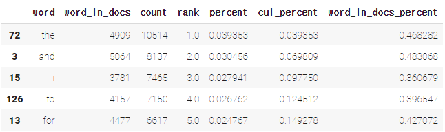
### 누적 분포 그래프 : cul_percent열 활용
import seaborn as sns

sns.lineplot(x='rank', y='cul_percent', data=wc);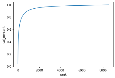
wc[wc['rank'] <= 1000]['cul_percent'].max()
>>> 0.9097585076280484
3) 시각화 : Squarify 라이브러리
!pip install squarify

import squarify
import matplotlib.pyplot as plt

# 등장 비율 상위 20개 단어
wc_top20 = wc[wc['rank'] <= 20]
squarify.plot(sizes=wc_top20['percent'], label=wc_top20['word'], alpha=0.6)
plt.axis('off')
plt.show()
토큰화2 : SpaCy
- 문서 구성요소를 다양한 구조에 나누어 저장하지 않고 요소를 색인화하여 검색 정보를 간단히 저장하는 라이브러리
- NLTK 라이브러리보다 더 빨라 최근에는 SpaCy 라이브러리를 많이 사용
- 공식 문서
# 필요한 모듈 import
import spacy
from spacy.tokenizer import Tokenizer

nlp = spacy.load("en_core_web_sm")

tokenizer = Tokenizer(nlp.vocab)


# 토큰화를 위한 파이프라인 구성

tokens = []

for doc in tokenizer.pipe(df['reviews.text']):
    doc_tokens = [re.sub(r"[^a-z0-9]", "", token.text.lower()) for token in doc]
    tokens.append(doc_tokens)

df['tokens'] = tokens
df['tokens'].head()
>>> 0    [though, i, have, got, it, for, cheap, price, ...
	1    [i, purchased, the, 7, for, my, son, when, he,...
	2    [great, price, and, great, batteries, i, will,...
	3    [great, tablet, for, kids, my, boys, love, the...
	4    [they, lasted, really, little, some, of, them,...
	Name: tokens, dtype: object
spacy의
tokenizer.pipe
- tokenizer 통과 : 단순 문자열이 아닌
spacy.tokens.doc.Doc형태로 변환- 자연어처리에 유용한 다양한 메소드 포함
type(tokenizer.pipe(df['reviews.text']))
>> generator
# A doc is a sequence of Token(<class 'spacy.tokens.doc.Doc'>) for doc in tokenizer.pipe(df['reviews.text']): print(doc) # 토큰(단어) 출력 for doc in tokenizer.pipe(df['reviews.text']): for token in doc: print(token)
# word_count 함수를 사용하여 단어의 분포 나타내기
wc = word_count(df['tokens'])
wc.head()
# squarify : SpaCy로 토큰화 한 문장에 대하여 등장 비율 상위 20개 단어의 결과 시각화
wc_top20 = wc[wc['rank'] <= 20]

squarify.plot(sizes=wc_top20['percent'], label=wc_top20['word'], alpha=0.6 )
plt.axis('off')
plt.show()
불용어(Stop words) 처리
- 갖고 있는 데이터에서 큰 의미가 없어 분석을 하는 것에 있어 큰 도움이 되지 않는 단어
- 조사, 접미사, 접속사, 관사, 부사, 대명사, 일반동사 등
- NLTK : 100여개 이상의 영어 단어들을 불용어로 패키지 내에서 미리 정의하고 있으며 개발자가 직접 정의할 수도 있다.
### spacy가 기본적으로 제공하는 불용어
print(nlp.Defaults.stop_words)
>>> {'by', 'may', 'five', 'afterwards', 'must', 'why', 'take', 'on', 'more', 'mostly', 'else'...


### 불용어 제외하고 토크나이징 진행한 결과
tokens = []
# 토큰에서 불용어 제거, 소문자화하여 업데이트
for doc in tokenizer.pipe(df['reviews.text']):
    doc_tokens = []

    # A doc is a sequence of Token(<class 'spacy.tokens.doc.Doc'>)
    for token in doc:
        # 토큰이 불용어와 구두점이 아니면 저장
        if (token.is_stop == False) & (token.is_punct == False):
            doc_tokens.append(token.text.lower())

    tokens.append(doc_tokens)

df['tokens'] = tokens
df.tokens.head()
>>> 0    [got, cheap, price, black, friday,, fire, grea...
    1    [purchased, 7", son, 1.5, years, old,, broke, ...
    2    [great, price, great, batteries!, buying, anyt...
    3         [great, tablet, kids, boys, love, tablets!!]
    4    [lasted, little.., (some, them), use, batterie...
    Name: tokens, dtype: object


wc = word_count(df['tokens'])
wc_top20 = wc[wc['rank'] <= 20]

squarify.plot(sizes=wc_top20['percent'], label=wc_top20['word'], alpha=0.6)
plt.axis('off')
plt.show()
# 불용어들이 모두 제거가 되어 완전히 다른 단어들이 상위에서 보임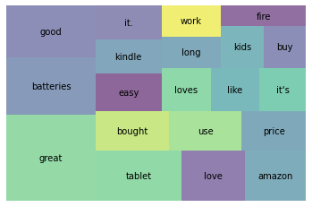
불용어 커스터마이징
다루는 데이터에 따라 불용어를 커스터마이즈할 수 있다. (추가와 제거 모두 가능)
STOP_WORDS = nlp.Defaults.stop_words.union(['batteries','I', 'amazon', 'i', 'Amazon', 'it', "it's", 'it.', 'the', 'this'])통계적 트리밍(Trimming)
불용어를 직접적으로 제거하는 대신 통계적인 방법을 통해 말뭉치 내에서 너무 많거나, 너무 적은 토큰을 제거하는 방법
### 단어들의 누적분포 그래프
sns.lineplot(x='rank', y='cul_percent', data=wc)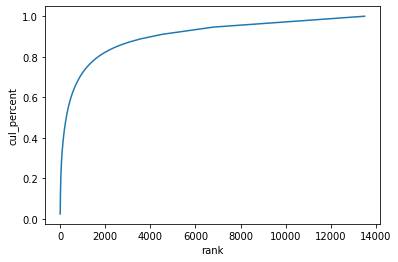 [그래프 해석]
- 자주 나타나는 단어들 (그래프의 왼쪽)
-> 여러 문서에 두루 나타나기 때문에 문서 분류 단계에서 통찰력을 제공하지 않음 - 자주 나타나지 않는 단어들 (그래프의 오른쪽)
-> 너무 드물게 나타나기 때문에 큰 의미가 없을 확률이 높음
# 자주 나타나지 않는 단어들 확인
wc.tail(20)

# 문서에 나타나는 빈도
sns.displot(wc['word_in_docs_percent'],kind='kde')
# 최소한 1% 이상 문서에 나타나는 단어들만 선택
wc = wc[wc['word_in_docs_percent'] >= 0.01]
sns.displot(wc['word_in_docs_percent'], kind='kde');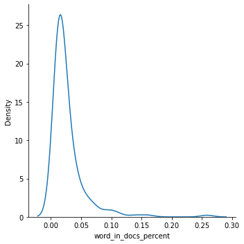
어간 추출(Stemming)과 표제어 추출(Lemmatization)
어간 추출(Stemming)
- 말뭉치의 복잡성을 줄여주는 텍스트 정규화 기법
- 단어로부터 어간(stem)을 추출하는 작업. 단어를 보고 어림짐작하여 어미를 잘라 어간을 추출하므로 표제어 추출보다 성능이 떨어진다.
- Stemming 방법에는 Porter, Snowball, Dawson 등의 알고리즘이 있다.
(*Spacy 는 Stemming을 제공하지 않고 Lemmatization만 제공)
-> A Comparative Study of Stemming Algorithms어간(stem)이란?
단어의 의미가 포함된 부분으로 접사등이 제거된 형태
어근이나 단어의 원형과 같지 않을 수 있다.
ex) argue, argued, arguing, argus의 어간 : 단어들의 뒷 부분이 제거된 argu
from nltk.stem import PorterStemmer

ps = PorterStemmer()

words = ["wolf", "wolves"]

for word in words:
    print(ps.stem(word))

>>> wolf
    wolv
=> Porter 알고리즘은 단지 단어의 끝 부분을 자르는 역할을 해서 사전에도 없는 단어가 많이 나오게 되지만 조금 이상하긴 해도 현실적으로 사용하기에 Stemming 은 성능이 나쁘지 않다. 알고리즘이 간단하여 속도가 빠르기 때문에 속도가 중요한 검색 분야에서 많이 사용한다.
아마존 리뷰데이터 stemming
### token -> stemming
tokens = []
for doc in df['tokens']:
    doc_tokens = []
    for token in doc:
        doc_tokens.append(ps.stem(token))
    tokens.append(doc_tokens)

df['stems'] = tokens


### top20
wc = word_count(df['stems'])
wc_top20 = wc[wc['rank'] <= 20]


### 시각화
squarify.plot(sizes=wc_top20['percent'], label=wc_top20['word'], alpha=0.6 )
plt.axis('off')
plt.show()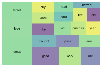
표제어 추출(Lemmatization)
- 말뭉치의 복잡성을 줄여주는 텍스트 정규화 기법
- 품사와 같은 문법적인 요소와 더 의미적인 부분을 감안하여 정확히 어근 단어를 찾아준다. 그래서 어간 추출보다 보다 많은 연산이 필요하기때문에 시간이 더 오래걸리지만 더 체계적이다. 이는 단어의 품사 정보를 알아야만 정확한 결과를 얻을 수 있다.
lem = "The social wolf. Wolves are complex."

nlp = spacy.load("en_core_web_sm")

doc = nlp(lem)

# wolf, wolve가 어떤 Lemma로 추출되는지 확인
for token in doc:
    print(token.text, "  ", token.lemma_)

>>> The    the
    social    social
    wolf    wolf
    .    .
    Wolves    wolf
    are    be
    complex    complex
    .    .
Stemming 에서는 wolf -> wolf, wolves -> wolv 로 변형되었지만,
Lemmatization에서는 wolf -> wolf, wolves -> wolf 로 변형되는 것을 볼 수 있다.
### Lemmatization 함수
def get_lemmas(text):

    lemmas = []

    doc = nlp(text)

    for token in doc:
        if ((token.is_stop == False) and (token.is_punct == False)) and (token.pos_ != 'PRON'):
            lemmas.append(token.lemma_)

    return lemmas

### 함수로 텍스트 데이터 정규화 진행
df['lemmas'] = df['reviews.text'].apply(get_lemmas)
df['lemmas'].head()

### top20 시각화
wc = word_count(df['lemmas'])
wc_top20 = wc[wc['rank'] <= 20]

squarify.plot(sizes=wc_top20['percent'], label=wc_top20['word'], alpha=0.6 )
plt.axis('off')
plt.show()
등장 횟수 기반의 표현 (Count-based Representation)
- 단어가 특정 문서(혹은 문장)에 들어있는 횟수를 바탕으로 해당 문서를 벡터화
- 대표적인 방법 : Bag-of-Words(TF, TF-IDF) 방식
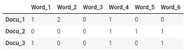
- 벡터화 된 문서는 문서-단어 행렬(각 행에는 문서(Document)가, 각 열에는 단어(Term)가 있는 행렬)의 형태로 나타내어진다.
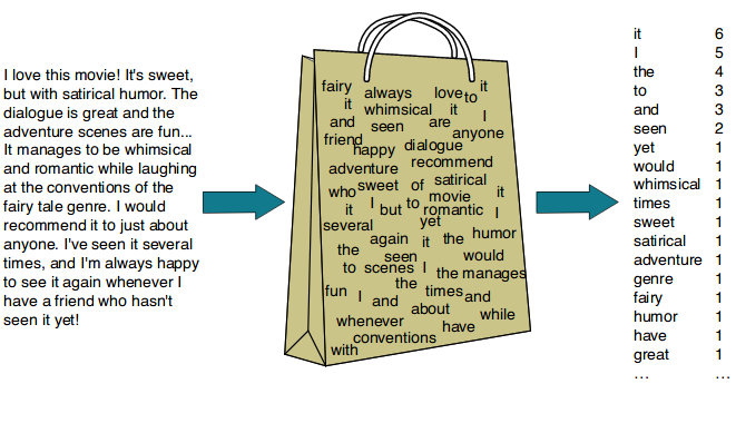
Bag-of-Words(BoW) : TF(Term Frequency)
- 가장 단순한 벡터화 방법 중 하나
- 문서(혹은 문장)에서 문법이나 단어의 순서 등을 무시하고 단순히 단어들의 빈도만 고려하여 벡터화
CountVectorizer: text
### Spacy 불러오기
# 모듈에서 사용할 라이브러리와 spacy모델 불러오기
import pandas as pd
import seaborn as sns
import matplotlib.pyplot as plt

from sklearn.feature_extraction.text import CountVectorizer, TfidfVectorizer
from sklearn.metrics.pairwise import cosine_similarity
from sklearn.neighbors import NearestNeighbors
from sklearn.decomposition import PCA

import spacy
nlp = spacy.load("en_core_web_sm")


### Bag-of-Words 예제
# 예제로 사용할 text 선언
text = """In information retrieval, tf–idf or TFIDF, short for term frequency–inverse document frequency, is a numerical statistic that is intended to reflect how important a word is to a document in a collection or corpus.
It is often used as a weighting factor in searches of information retrieval, text mining, and user modeling.
The tf–idf value increases proportionally to the number of times a word appears in the document and is offset by the number of documents in the corpus that contain the word,
which helps to adjust for the fact that some words appear more frequently in general.
tf–idf is one of the most popular term-weighting schemes today.
A survey conducted in 2015 showed that 83% of text-based recommender systems in digital libraries use tf–idf."""


# spacy의 언어모델을 이용하여 token화된 단어들 확인
doc = nlp(text)

# 불용어와 구두점 제거
print([token.lemma_ for token in doc if (token.is_stop != True) and (token.is_punct != True)])
#>>> ['information', 'retrieval', 'tf', 'idf', 'TFIDF', 'short', 'term', 'frequency'...


from sklearn.feature_extraction.text import CountVectorizer

# 문장으로 이루어진 리스트 저장
sentences_lst = text.split('\n')
#>> ['In information retrieval, tf–idf or TFIDF, short for term frequency–inverse document frequency,...

# CountVectorizer를 변수에 저장
vect = CountVectorizer()

# 어휘 사전 생성
vect.fit(sentences_lst)
""">>> CountVectorizer(analyzer='word', binary=False, decode_error='strict',
                dtype=<class 'numpy.int64'>, encoding='utf-8', input='content',
                lowercase=True, max_df=1.0, max_features=None, min_df=1,
                ngram_range=(1, 1), preprocessor=None, stop_words=None,
                strip_accents=None, token_pattern='(?u)\\b\\w\\w+\\b',
                tokenizer=None, vocabulary=None)"""

# text를 DTM(document-term matrix)으로 변환(transform)
dtm_count = vect.transform(sentences_lst)
dtm_count  # sparse matrix
""">>> <6x75 sparse matrix of type '<class 'numpy.int64'>'
	with 108 stored elements in Compressed Sparse Row format>"""

# vocabulary(모든 토큰)와 맵핑된 인덱스 정보 확인
vect.vocabulary_
"""
>>> {'2015': 0,
 '83': 1,
 'adjust': 2,
 'and': 3,
 'appear': 4,
 'appears': 5,
 'as': 6,
 'based': 7,
 .
 .
 .
 """

 # 추출된 토큰 나열
 print(f"""
features : {vect.get_feature_names()}  # vect = 어휘사전
num of features : {len(vect.get_feature_names())}
""")
""">>> features : ['2015', '83', 'adjust', 'and', 'appear'...
	num of features : 75"""
# dtm_count.shape => (6, 75)

# CountVectorizer로 제작한 dtm 분석
print(type(dtm_count))
print(dtm_count)
#>>> <class 'scipy.sparse.csr.csr_matrix'>
    """
    CSR(Compressed Sparse Row matrix)
    : 행렬의 값이 대부분 '0'인 희소행렬(Sparse matrix)을 가로의 순서대로 재정렬하는 방법으로 행에 관여하여 정리 압축한 것
    * https://rfriend.tistory.com/551

    print(dtm_count) => (i번째 document, j번째 단어)  등장 횟수
    """
    (0, 9)	1
    (0, 12)	1
    (0, 14)	2
    (0, 18)	1
    (0, 19)	2
    (0, 23)	1
    (0, 24)	1
     :	 :

# .todense() 메서드 : numpy.matrix 타입으로 돌려줌

print(type(dtm_count))
print(type(dtm_count.todense()))
dtm_count.todense()
"""
>>> <class 'scipy.sparse.csr.csr_matrix'>
    <class 'numpy.matrix'>
    matrix([[0, 0, 0, 0, 0, 0, 0, 0, 0, 1, 0, 0, 1, 0, 2, 0, 0, 0, 1, 2, 0,
             0, 0, 1, 1, 1, 2, 0, 1, 1, 1, 3, 0, 0, 0, 0, 0, 0, 0, 1, 0, 0,
             0, 0, 2, 0, 0, 0, 1, 1, 0, 0, 1, 0, 0, 1, 0, 0, 1, 0, 1, 1, 1,
             0, 0, 2, 0, 0, 0, 0, 0, 0, 0, 1, 0],
            [0, 0, 0, 1, 0, 0, 1, 0, 0, 0, 0, 0, 0, 0, 0, 0, 0, 1, 0, 0, 0,
             0, 0, 0, 0, 0, 1, 0, 1, 0, 0, 1, 1, 0, 1, 1, 0, 0, 0, 0, 1, 0,
             1, 0, 0, 0, 0, 0, 0, 1, 0, 1, 0, 0, 0, 0, 0, 0, 0, 1, 0, 0, 0,
             0, 0, 0, 0, 0, 1, 1, 0, 1, 0, 0, 0],
             .
             .
             .

# DataFrame으로 변환한 후에 결과값 확인
dtm_count = pd.DataFrame(dtm_count.todense(), columns=vect.get_feature_names())
print(type(dtm_count))
#>>> <class 'pandas.core.frame.DataFrame'>

dtm_count
CountVectorizer: 아마존 리뷰 데이터
from sklearn.feature_extraction.text import CountVectorizer

count_vect = CountVectorizer(stop_words='english', max_features=100)  # top100
# max_features : corpus중 빈도수가 가장 높은 n개의 단어만 추출, feature space 차원 조절

# Fit 후 dtm 만들기(문서, 단어마다 tf-idf 값 계산)
dtm_count_amazon = count_vect.fit_transform(df['reviews.text'])

# dataframe으로 만들기
dtm_count_amazon = pd.DataFrame(dtm_count_amazon.todense(), columns=count_vect.get_feature_names())
dtm_count_amazon
Bag-of-Words(BoW) : TF-IDF (Term Frequency - Inverse Document Frequency)
- 다른 문서에 등장하지 않는 단어, 즉 특정 문서에만 등장하는 단어에 가중치를 두는 방법
TF-IDF의 수식
- = 특정 문서 내 단어 의 수
- 분류 대상이 되는 모든 문서의 수 :
- 단어 w가 들어있는 문서의 수 :
*log를 취해줄 경우 : scaling의 효과, 가중치가 너무 많이 차이 나는 것 막음
(TfidVectorizer : 밑이 e인 자연로그 사용)
TfidfVectorizer: text
sentences_lst
"""
>>> ['In information retrieval, tf–idf or TFIDF, short for term frequency–inverse document frequency, is a numerical statistic that is intended to reflect how important a word is to a document in a collection or corpus.',
 'It is often used as a weighting factor in searches of information retrieval, text mining, and user modeling.',
 'The tf–idf value increases proportionally to the number of times a word appears in the document and is offset by the number of documents in the corpus that contain the word,',
 'which helps to adjust for the fact that some words appear more frequently in general.',
 'tf–idf is one of the most popular term-weighting schemes today.',
 'A survey conducted in 2015 showed that 83% of text-based recommender systems in digital libraries use tf–idf.']
"""

# TF-IDF vectorizer
# 테이블을 작게 만들기 위해 max_features=15로 제한
tfidf = TfidfVectorizer(stop_words='english', max_features=15)

# Fit 후 dtm 만들기(문서, 단어마다 tf-idf 값 계산)
dtm_tfidf = tfidf.fit_transform(sentences_lst)

# dataframe 만들기
dtm_tfidf = pd.DataFrame(dtm_tfidf.todense(), columns=tfidf.get_feature_names())
dtm_tfidf
*(비교) CountVectorizer를 사용하여 생성한 DTM의 값

파라미터 튜닝
# SpaCy 를 이용한 Tokenizing

def tokenize(document):
    doc = nlp(document)
    return [token.lemma_.strip() for token in doc if (token.is_stop != True) and (token.is_punct != True) and (token.is_alpha == True)

"""
    args:
        stop_words : 'english'->영어용 스탑 워드 사용, list, or None (default)

        ngram_range = (min_n, max_n), min_n 개~ max_n 개를 갖는 n-gram(n개의 연속적인 토큰)을 토큰으로 사용합니다.
        ex) ngram_range=(1,3) -> 각 단어 하나하나 뿐만 아니라 연속된 3개 단어까지를 하나의 토큰으로 생성

        *DF(document_frequency) : "문서"의 수
        min_df = n : int, 최소 n개의 문서에 나타나는 토큰만 사용합니다. / DF의 최소값을 설정하여 해당 값보다 작은 DF를 가진 단어들은
                        단어사전 (vocabulary_)에서 제외하고, 인덱스 부여X
        max_df = m : float(0~1), m * 100% 이상 문서에 나타나는 토큰은 제거합니다.
        max_feature : tf-idf vector의 최대 feature를 설정해주는 파라미터

        파라미터 : https://chan-lab.tistory.com/27
    """

tfidf_tuned = TfidfVectorizer(stop_words='english'
                        ,tokenizer=tokenize
                        ,ngram_range=(1,2)
                        ,max_df=.7
                        ,min_df=3
                       )

dtm_tfidf_tuned = tfidf_tuned.fit_transform(df['reviews.text'])
dtm_tfidf_tuned = pd.DataFrame(dtm_tfidf_tuned.todense(), columns=tfidf_tuned.get_feature_names())
dtm_tfidf_tuned.head()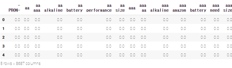
❓n-gram이란?
n개의 연속적인 단어 나열로 갖고 있는 코퍼스에서 n개의 단어 뭉치 단위로 끊어서 이를 하나의 토큰으로 간주하여 단어의 순서를 무시하는 bag of words의 단점을 보완한다.
예를 들어서 문장 An adorable little boy is spreading smiles이 있을 때, 각 n에 대해서 n-gram을 전부 구해보면 다음과 같다.
- unigrams : an, adorable, little, boy, is, spreading, smiles
- bigrams : an adorable, adorable little, little boy, boy is, is spreading, spreading smiles
- trigrams : an adorable little, adorable little boy, little boy is, boy is spreading, is spreading smiles
- 4-grams : an adorable little boy, adorable little boy is, little boy is spreading, boy is spreading smiles
https://velog.io/@ny_/n-gram
https://wikidocs.net/21692
TfidfVectorizer: 아마존 리뷰 데이터
tfidf_vect = TfidfVectorizer(stop_words='english', max_features=100)

# Fit 후 dtm 만들기(문서, 단어마다 tf-idf 값을 계산합니다)
dtm_tfidf_amazon = tfidf_vect.fit_transform(df['reviews.text'])

# dataframe 만들기
dtm_tfidf_amazon = pd.DataFrame(dtm_tfidf_amazon.todense(), columns=tfidf_vect.get_feature_names())
dtm_tfidf_amazon
❗️
CountVectorizervsTfidfVectorizer
CountVectorizer
: 텍스트에서 단위별 등장횟수를 카운팅하여 수치벡터화 하는 것
(단위 : 정하는대로. 가장 많이 사용되는 것은 단어 단위의 카운팅)
TfidfVectorizer
: 모든 문서에서 자주 등장하는 단어에는 페널티를 주고, 해당 문서에서만 자주 등장하는 단어에 높은 가중치를 주는 방식
- 특정 문서에 등장하는 단어 -> 가중치 (ex.식단표의 '깐풍기, 카레'/ '밥, 우유'(X))
- 그렇게 함으로써 해당 단어가 실질적으로 중요한 단어인지 검사하는 것
유사도를 이용한 문서 검색

네이버, 구글과 같은 검색엔진은 검색어(Query, 쿼리)와 문서에 있는 단어(Key,키)의 매칭(Matching)을 통해 동작한다.
여러가지 매칭의 방법들 중 가장 클래식한 방법은 "유사도 측정 방법"이다.
코사인 유사도(Cosine Similarity)
- 가장 많이 쓰이는 유사도 측정 방법
- 두 벡터가 이루는 각의 코사인 값을 이용하여 구할 수 있는 유사도('두 벡터가 가리키는 방향이 얼마나 비슷한가')

- 두 벡터(문서)가
- 완전히 같을 경우
- 90도의 각을 이루면
- 완전히 반대방향을 이루면
NearestNeighbor (K-NN, K-최근접 이웃)
K-최근접 이웃법은 쿼리와 가장 가까운 상위 K개의 근접한 데이터를 찾아서 K개 데이터의 유사성을 기반으로 점을 추정하거나 분류하는 예측 분석에 사용된다.
from sklearn.neighbors import NearestNeighbors

# dtm을 사용히 NN 모델을 학습시킵니다. (디폴트)최근접 5 이웃.
nn = NearestNeighbors(n_neighbors=5, algorithm='kd_tree')
nn.fit(dtm_tfidf_amazon)

# 2 번째 인덱스에 해당하는 문서와 가장 가까운 문서 (0 포함) 5개의 거리(값이 작을수록 유사합니다)와 문서의 인덱스
nn.kneighbors([dtm_tfidf_amazon.iloc[2]])
"""
>>> (array([[0.        , 0.64660432, 0.73047367, 0.76161463, 0.76161463]]),
 array([[   2, 7278, 6021, 1528, 4947]]))
"""

print(df['reviews.text'][2][:300])
print(df['reviews.text'][7278][:300])
"""
>>> Great price and great batteries! I will keep on buying these anytime I need more!
    Always need batteries and these come at a great price.
"""

>### 문서 검색 예제

```python
# 출처 : https://www.amazon.com/Samples/product-reviews/B000001HZ8?reviewerType=all_reviews
sample_review = ["""in 1989, I managed a crummy bicycle shop, "Full Cycle" in Boulder, Colorado.
The Samples had just recorded this album and they played most nights, at "Tulagi's" - a bar on 13th street.
They told me they had been so broke and hungry, that they lived on the free samples at the local supermarkets - thus, the name.
i used to fix their bikes for free, and even feed them, but they won't remember.
That Sean Kelly is a gifted songwriter and singer."""]

# 학습된 **`TfidfVectorizer`** 를 통해 Sample Review 변환
new = tfidf_vect.transform(sample_review)

nn.kneighbors(new.todense())

# 가장 가깝게 나온 문서 확인
df['reviews.text'][10035]
🧐 Review
-
자연어처리
-
벡터화
- 등장 횟수 기반 표현 (Count-based Representation)
- 분포 기반 표현 (Distributed Representation)
-
전처리(Preprocessing)
- 토큰화(Tokenization) : 대소문자 통일, 정규표현식
- 불용어(Stop words)
- 어간 추출(Stemming)과 표제어 추출(Lemmatization)
-
등장 횟수 기반의 표현(Count-based Representation)
- 문서-단어 행렬(Document-Term Matrix, DTM)
- Bag-of-words : TF (Countvectorizer)
- TF-IDF (Tfidfvectorizer)