AI/ML/DL (1) - k-nearest neighbors algorithm

xsldihsl·2024년 4월 4일

K-Nearest Neighbors KNeighborsClassifier ML algorithm machine learning

AI/ML/DL

목록 보기

1/25

이번 글에서는 supervised machine learning 중 간단한 k-nearest neighbors algorithm 를 이용한 classification 을 수행해보겠다.

AI, Machine learning, and Deep learning
k-nearest neighbors algorithm
KNeighborsClassifier
train_test_split
Data preprocessing

1. AI, Machine learning, and Deep learning

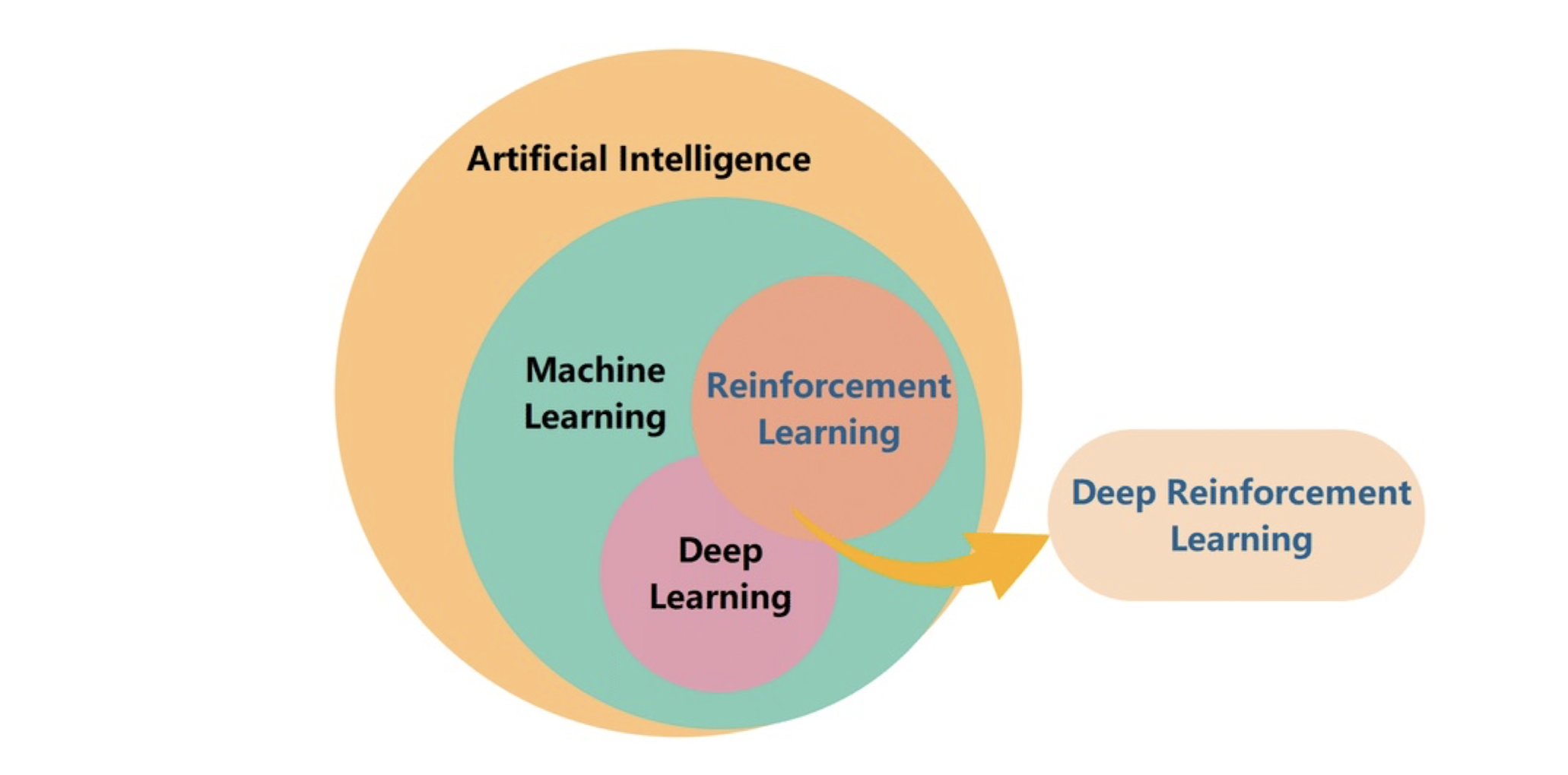
Machine learning (ML) 은 AI 의 하위 분야로서 여러 알고리즘을 포함하고 있는데, 이 수많은 알고리즘 중 "인공신경망", 즉 artificial neural network 를 이용하는 것들을 Deep learning (DL) 로 분류하고 있다. 그 예로는 TensorFlow (Keras API) 나 PyTorch 같은 것이 있다.

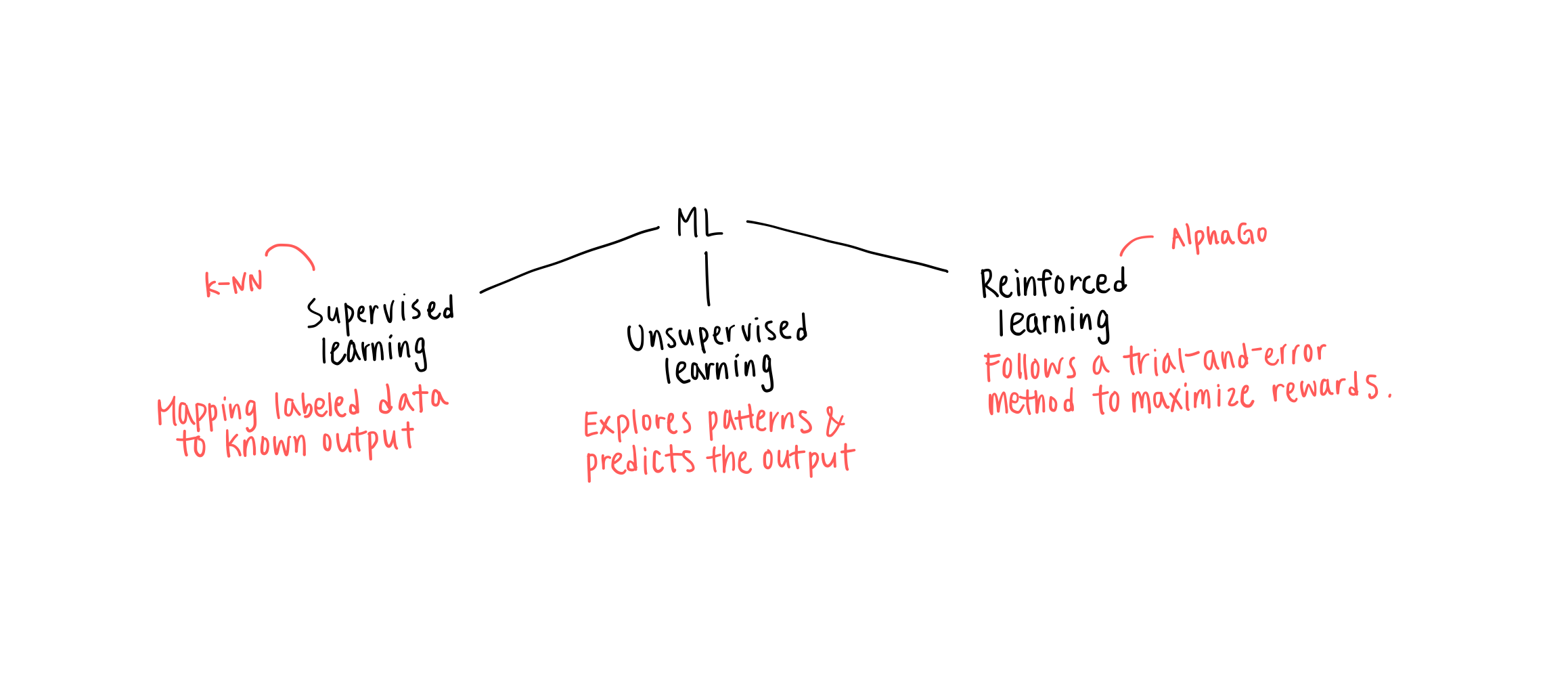
위와 같이 ML 은 학습 알고리즘에 따라 세 가지로 구분할 수 있다.

Supervised learning: Input 과 target 이 있는 데이터 상에서 학습하는 알고리즘
Unsupervised learning: Target 데이터 없이 input 만 제공될 때 패턴에 따라 특정 작업 수행
Reinforced learning: 수행 결과에 따른 주변 환경의 피드백을 받아 계속 개선해나가는 알고리즘

특히 오늘 중점적으로 다룰 supervised learning 은 "classification" 과 "regression" 으로 나눌 수 있다.

2. k-nearest neighbors algorithm

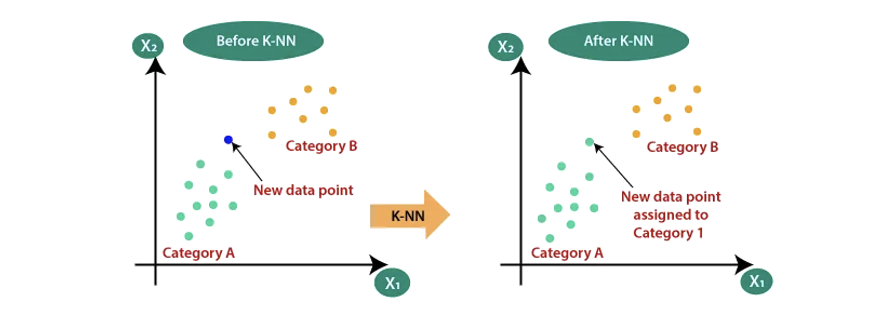
먼저 지도학습의 classification 을 알아보자. 두 개의 class 가 있을 때 이를 분류하는 것을 binary classification 이라고 한다. 이 때, 각각의 object 는 "sample" 이라고 하며, 그것이 가지는 특성들은 "features" 라고 한다 (예: 길이, 무게 등). 이진 분류를 위해 우리는 간단하고 단순한 k-nearest neighbors (k-NN) 알고리즘을 이용해 볼 것이다.

k-NN is a non-parametric supervised learning method used for classification and regression. The input consists of the k closest training samples in a data set.

k-NN 은 간단히 말해 주변에 가까운 데이터들을 토대로 결과를 도출하는 것이다. 이 "결과"라 함은 classification 에서는 어떤 class 에 포함되는지를, 그리고 regression 에서는 어떠한 특성의 value 를 의미한다.

3. KNeighborsClassifier

k-NN classification 을 위해 sklearn 의 neighbors module 이 제공하는 KNeighborsClassifier 를 이용할 것이다. 기본적으로 KNeighborsClassifier 가 참고하는 샘플들은 5 개인데 우리는 "n_neighbors" 라는 parameter 를 통해 이웃의 개수를 특정해 줄 수도 있다. 그렇다면 길이와 무게를 바탕으로 주어진 샘플이 어떤 채소일지 예측해보자.

squash_length = [25.4, 26.3, ...]
squash_weight = [242.0, 290.0, ...]

chilli_length = [9.8, 10.5, ...]
chilli_weight = [6.7, 7.5, ...]

이처럼 squash 와 chilli 의 길이, 무게가 각각 주어졌을 때, 분류를 위해 우리는 이를 하나의 데이터로 모아야 한다. 35 개의 squash 샘플들과 14 개의 chilli 샘플들이 주어졌다면 이후에 우리는 squash 를 1 로, chilli 를 0 으로 나타내어 target 을 지정해 줄 것이며, 학습한 모델을 이용해 길이 25 cm, 무게 250 g 인 채소 샘플의 class 를 예측해 볼 것이다.

veggie_length = squash_length + chilli_length
veggie_weight = squash_weight + chilli_weight

현재까지 정의된 veggie_length 와 veggie_weight 은 <class 'list'> 이다. 하지만 sklearn 은 각각의 특성들이 column 에 담긴 2-dim. array 를 요구하기 때문에 Numpy 를 이용해 변환해주자.

veggie_data = np.column_stack((veggie_length, veggie_weight))
veggie_target = np.concatenate((np.ones(35), np.zeros(14))

참고로 Numpy 는 python 의 대표적인 배열 라이브러리로서 배열 연산에 유용한 함수들을 많이 가지고 있다.

Numpy supports for large, multi-dimensional arrays and matrices, along with a large collection of high-level mathematical functions to operate on these arrays.

4. train_test_split

ML model 을 훈련시키고 시험해보기 위해서는 training 그리고 test, 이렇게 두 개의 data sets 가 필요하다. 이 때 우리는 어느 한 쪽에 특정 샘플들이 치우쳐 들어가있지 않도록 "sampling bias" 에 주의해야 한다. 이를 방지하며 train set 과 test set 을 나누기 위해 sklearn 의 model_selection 에는 "train_test_split" 이라는 함수가 존재한다. 또한 이 함수의 parameters 중 "stratify" 는 specify 된 array 를 class label 로 삼아 샘플들이 더욱 골고루 나뉘도록 도와준다.

from sklearn.neighbors import KNeighborsClassifier
from sklearn.model_selection import train_test_split

train_input, test_input, train_target, test_target = train_test_split(veggie_data, veggie_target, stratify = veggie_target)
kn = KNeighborsClassifier()
kn.fit(train_input, train_target)
kn.score(test_input, test_target)
kn.predict([[25,150]])

위와 같이 우리는 train set 으로 "kn" 이라는 모델을 학습시키고 test set 을 이용해 성능을 검증해보았다. Classification 에서 score function 은 "accuracy" 를 보여준다. 좀 더 직관적으로 class membership 을 판단하기 위해 아래와 같이 scatter plot 을 이용하였다.

(a) x 축의 domain 과 y 축의 range 가 달라 직접적인 비교가 불가하다.
(b) x 축의 domain 을 y 축의 range 에 맞췄더니 weight 에 지나치게 의존적이다.
(c) 단, 위와 같은 이유로 x 와 y 축의 scaling 을 맞추기 위한 data processing 을 필요로 하게 되었다.

5. Data preprocessing

The process of detecting, correcting, or removing corrupt or inaccurate records from a dataset. While the needs vary, almost every model requires a sort of preprocessing.

대부분의 모델들은 데이터 전처리라 불리는 과정을 어느정도 기본적으로 요구한다. 이에 대표적으로 쓰이는 것이 바로 "standard score" 또는 "z-score" 이다. 다음의 formula 에서도 알 수 있듯이 z-score 를 구하기 위해 우리는 mean 과 stdev 를 구해야하는데, 앞서 소개했던 numpy 의 함수들을 이용하면 편리하다.

The z-score measures exactly how many standard deviations above or below the mean a data point is.

$z = \frac{data point - mean}{stdev}$

import numpy as np

mean = np.mean(train_input, axis=0)
std = np.std(train_input, axis=0)

train_scaled = (train_input - mean)/std
kn.fit(train_scaled, train_target)
test_scaled = (test_input - mean)/std
kn.score(test_scaled, test_target)
new = ([25,150] - mean)/std
print(kn.predict([new]))

# Scatter plot
distances, indices = kn.neighbors([new])

plt.scatter(train_scaled[:,0], train_scaled[:,1])
plt.scatter(new[0], new[1], marker='^')
plt.scatter(train_scaled[indices,0], train_scaled[indices,1], marker='D')
plt.xlabel('length')
plt.ylabel('weight')
plt.show()

참고 링크: sklearn 의 KNeighborsClassifier 에 대한 설명과 parameters 제공
https://scikit-learn.org/stable/modules/generated/sklearn.neighbors.KNeighborsClassifier.html

참고 링크: k-nearest neighbors algorithm 에 관한 설명
https://en.wikipedia.org/wiki/K-nearest_neighbors_algorithm

xsldihsl

다음 포스트