5. Quasi-Newton Method for IK

SYiee·2023년 8월 7일

IK animation

Inverse Kinemtics (human animation)

목록 보기

5/7

🖤Introduction🖤

📌Quasi-Newton Methods

보통 이차 미분을 이용하는 method가 수렴이 더 빠르다.
→ it can be very expensive to calculate and store the inverse of the Hessian matrix at each iteration
→ 이차미분(헤시안)을 하는 것 자체가 굉장히 computational cost가 크다.

그래서 quasi-newton methods to approximate the Hessian 를 사용하게 된다.
→ 헤시안을 정확히 구하는 대신 approximate한다.

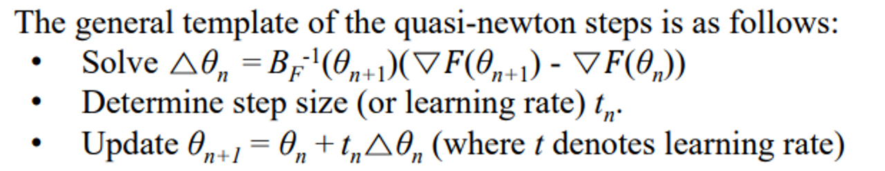
Quasi-Newton Computation flow:

Start with an initial guess for the optimal solution.
Compute the gradient at the current point.
Approximate the Hessian matrix or its inverse.
Update the solution using the approximated Hessian matrix.
Repeat steps until a stopping criterion is met (reaching a maximum number of iterations or a desired level of convergence.)

📌Quasi-Newton VS. Newton method.

Advantages

Reduced computational complexity.
Faster Convergence (especially for ill-conditioned problems).
빠르게 수렴한다
More robust as Quasi-Newton methods are less sensitive to the initial guess and can handle non-quadratic objective functions. 초기값의 상태에 조금 덜 민감하다. objective functions이 quadratic 하게 풀리지 않는다고 하더라도 괜찮다

Disadvantages

Less accurate Hessian matrix.
뉴턴 메서드 비해 정확도가 떨어진다
Slower convergence for some problems (when the approximations are not sufficiently accurate or when the problem is well-conditioned, the Newton method can converge more quickly than Quasi-Newton methods).
→ 초기값 자체가 이미 뉴텀 메서드로 충분히 수렴한 가능한 상태로 well conditioned되어 있는 상태에서는 굳이 쓸 필요가 없다. approximation이 들어가기 때문에 이게 잘 되지 않으면 충분한 성능을 내지 못한다. 실제로 아크로바틱한 동작에서는 잘 안되기도 한다.

🌊 Recent research topics:

Improves hessian approximations.

Parallelization and distributed computing.

Application to machine learning.

Understanding the convergence properties and establishing better stopping criteria.

🖤Basics🖤

📌Ill-conditioned problem

헤시안 매트릭스의 condition number 가 너무 크면 numerically challenging하게 만든다
- condition number : ratio of its largest and smallest eigenvalues
  eigenvalues 의 비율차이가 너무 클 때
  
  → 벡터에 매트릭스를 곱하는 것이 Transform(회전 + 늘리는 것)을 의미했었다. 이때 가하는 힘을 e1, e2이렇게 나누어 표현했는데 만약 e1이 엄청 크고 e2가 엄청 작다면, e1가 가까운 쪽으로 움직이면 변화율이 엄청 크고 반대는 엄청 작다.
  
  → 분명 같은 timestamp로 움직이는데 한쪽 축으로는 팍 움직이게 된다.
  
  → delta x를 얼마나 설정하게 되느냐에 따라 수렴을 할 수 있을지 없을지 결정되는데 그래프의 변화율이 너무 커진다.

🌊 This can arise from various sources:

Poor scaling of variables
- f(x,y) → x y가 scaling이 잘 못 됨.
- ex) 데이터를 인풋으로 넣어서 학습을 시키는데 어떤 것은 0-1000사이에 분포 0-100000000사이에 분포하는데 같은 파라미터로 두고 찾으면 안 찾아진다.
High-dimensional problems.
- 너무 많은 파라미터를 쓰면 파라미터들 사이에 eigenvalue가 다양화되니
Intrinsic properties of the objective function.
- 오브젝트 함수가 이미 그럴 수 밖에 없는 상황들이 있다.

🌊 This can be mitigated by using:

scaling을 잘 한다
Preconditioning
ill-condition에 robost한 alrorithm을 사용한다

📌 Definite Matrix

한 마디로 그냥 명칭이다.

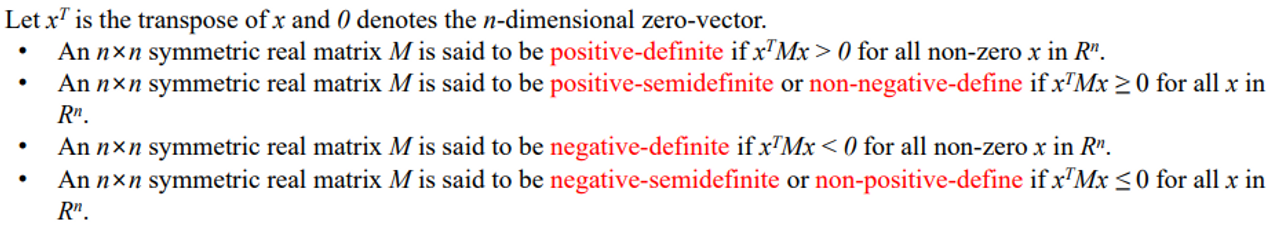
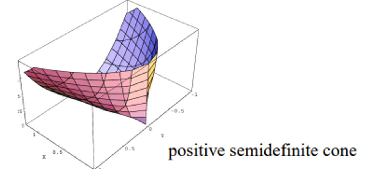
Positive-definite and positive-semidefinite은 convex optimization이라는 것에 기본이 된다

→ 포인트 p에서 헤시안 매트릭스가 양수이면 이 함수는 p에서 convex하다

→ p로 수렴한다는 것을 보장할 수 있다. itertative를 돌면 더 나은 해를 찾을 수 있는 것이 보장된다.

🌊 Definite matrix의 용도

Definite matrices are important in optimization problems
→ curvature of the objective function를 제공하기 때문
→ 이 문제가 풀 수 있는지 없는지 판단할 때 이것이 positive인지 negative인지 판단하면 얼추 맞는다. 즉 많은 계산을 사전에 하지 않고도 문제가 풀리지 풀리지 않을 지 판단이 가능해진다.

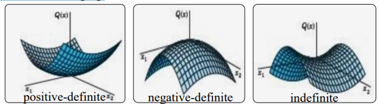
The properties of positive-definite matrix M include

1) all eigenvalues are positive
2) the matrix is invertible (역행렬가능)
3) the matrix is symmetric
- positive definite matrice는 convex functions에 매칭이 되고
- 하나의 global minimum 값을 갖는다
  
  ⇒ optimization 문제가 하나의 해를 갖는 것을 보장한다

The properties of negative-definite matrix M include

1) all eigenvalues are negative
2) the matrix is invertible
3) the matrix is symmetric.
- 반대로 위쪽에 도달
그림에서 indefinite(3번째) 경우

반드시 글로벌 미니멈이나 맥시멈으로 도달한다는 보장이 없다.

⇒ 문제를 optimization problem으로 풀 수 있을지도 없을지도 모를 때 definite matrix 성질을 이용해 미리 판단할 수 있다.

📌 Secant Method

root finding 알고리즘이다.

→ 뉴턴 메소드랑 비슷한 느낌을 가진다.
two previous points 를 이용해서 현재 추정중인 것의 일차 미분을 추정한다,
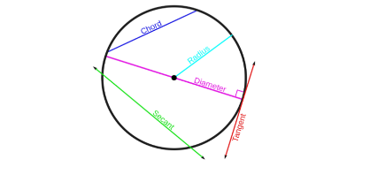
secant : 커브에서 두개의 distinct 포인트를 연결한 하나의 선을 말한다.
→ 원에서 지름을 지나지 않는 선

🌊일차 미분을 구할 수 없을 때 사용한다.
→ 함수 자체가 불가하거나 computational cost 때문에
→ 점 두개 이용해서 x증가량 y증가량 이용해서 마치 미분처럼 구할 수 있다.
→ 이차로 넘어가면 이전 두개 점에서의 일차미분과 값들을 이용해 구할 수 있다.

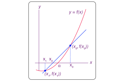
continuous function f(x)

the goal is to find a root of the function
두개의 initial guess가 있다.
iterative하게 돌면서 값을 찾아나간다

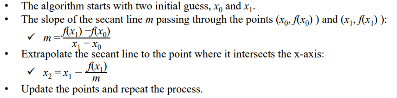
recurrence relation

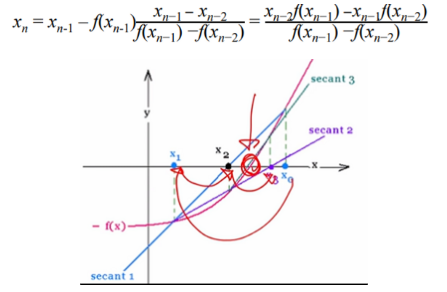
📌 Frobenius norm

The Frobenius norm, also known as the Euclidean norm, is a matrix norm that is used to measure the size of a matrix

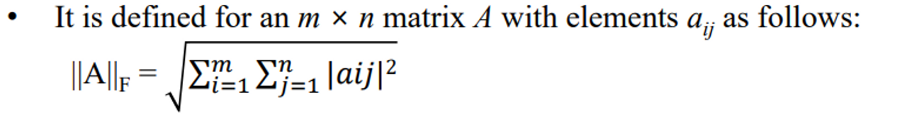
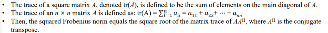
The Frobenius norm has a relationship with trace properties
- tr(A) : 매트릭스의 대각성분을 전부 더한 것
- 아래 식과같은 성질을 가지고 있다.
  real number로 오게 되면 conjugate가 사라지면서 $A^H = A^T$ 가 된다.

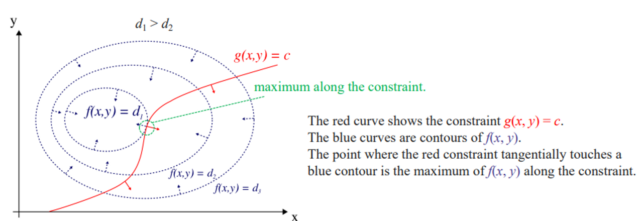
📌 Lagrange Multiplier

Lagrange multiplier 은 optimization problem에 사용되는데 어떤 constraint가 function에 가해지는 상황에서의 최소와 최댓값을 찾는 것이다.
→ 이전에 어떤 함수를 그냥 optimization할 때는 함수만 미분을 했었는데 거기에 어떤 constraint가 걸렸을 때 최적화 문제를 푸는 것이다.

Lagrange multipliers 가 오브젝티브 함수에 적용
맥시멈 포인트를 찾고 있다면 등고선이어서 가운데로 갈 수록 값이 커진다.

→ g(x,y)로 constraint를 건다. 이 빨간선 위로는 넘어오면 안된다고 정하는 것이다.

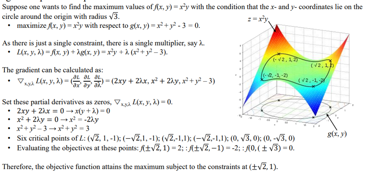
🌊 method overview

f의 최대나 최소를 구하는 것이 목표이다.

아래와 같이 쓸 수 있다.

각각에 대해(3개) 모두 편미분을 한다. 그리고 이것을 모두 0으로 만드는 critical point를 찾는다.

그리고 식을 풀어 optimal values for x and λ, y를 찾는다
구한 값들을 다시 함수f에 넣어 맥시멈 혹은 미니멈 값을 찾는다

⇒ multivariate 문제는 다루지 않는다. 너무 어렵기 때문^^

🖤Quasi-Newton Method🖤

ill-conditioned problem도 배우고 수렴하는지 수렴하지 않는지 사용하기 위해 Difinite Matirx도 배우고 secant method 이전 두 점의 일차 미분을 이용해 이차미분을 구할 수 있다는 것을 위에서 다루었다. Quasi-Newton을 수학적으로 정리하기 위해 필요한 Frobenius norm , Lagrange Multiplier 도 배웠다. 이 내용을 바탕으로 Quasi-Newton Method를 설명하고자 한다.

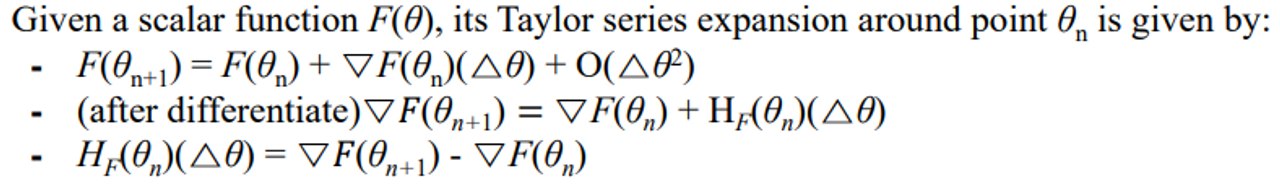
📌Search for extrema (optimization problem)

어떤 함수의 gradient = 0 이되는 점을 즉 일차 미분이 0이 되는 점을 찾는 것이다.
- $g = ▽f$
- $J(g) = H(f)$ (Recall that $J[▽f(x)] = H[f(x)]$ ).
optimum region 근처에서는 Quadratic적으로 approximartion이 가능하기 때문에 수렴이 가능하다. 그렇기에 그 점 근처에서 gradient와 Hessian을 사용해서 그 쪽으로 향하도록 한다.
→ 여기 분모에 들어가는 헤시안을 approximation 할 것이다.
→ 다시 구하는 것이 아닌 이전에 구한 $H_F(θ_{n-1})$ 을 사용해 헤시안을 업데이트 한다. 이를 통해 코스트를 줄일 것이다.

How to approximate the Hessian matrix?

positive-definite matrix B를 이용한다.
이를 오브젝티브 함수의 그라디언트 정보를 이용해 업데이트 한다.
secant equation plays a crucial role in computing Hessian approximation based on the gradient information

헤시안 매트릭스가 $θ_n , θ_{n+1}$ 사이에서 거의 constant하다고 가정하면 바로 식을 넣을 수 있다. “헤시안 거의 비슷하지 않을까?” 하고 그냥 넣어버리는 데 정확하지 않은 헤시안을 뜻하기 위해 B로 표기

아래것들을 만족하게 된다.

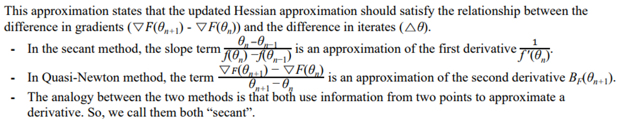
아래 문제를 풀게 된다.

⇒ 여기까지는 Hessian Matrix를 일차미분 gradient로 부터 계산해내는 방법을 이야기 했다.

이전 스텝의 Hessian을 사용해서 현재 Hessian을 업데이트 하는 방법론

There are several algorithms for updating B

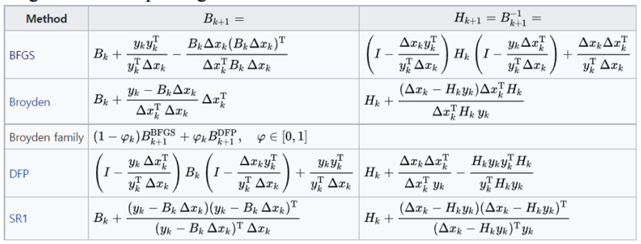
Broyden-Fletcher-Goldfarb-Shanno Method

BFGS은 최종보스이다.
- Positive definiteness : 결국 수렴할 수 밖에 없다
  ex) SR1은 이것이 보장이 되지 않아 어떤 함수에서는 발산한다.
- Convergence 가 빠르다
- Numerical stability
  → SR1은 ill-conditioned Hessian approximations, which can cause
  numerical difficulties.

하지만 학부생 수준에서 다루기에는 어렵기 때문에 BFGS의 기본이 되는 Broyden Method Derivation를 다루도록 한다.

🖤Broyden Method Derivation🖤

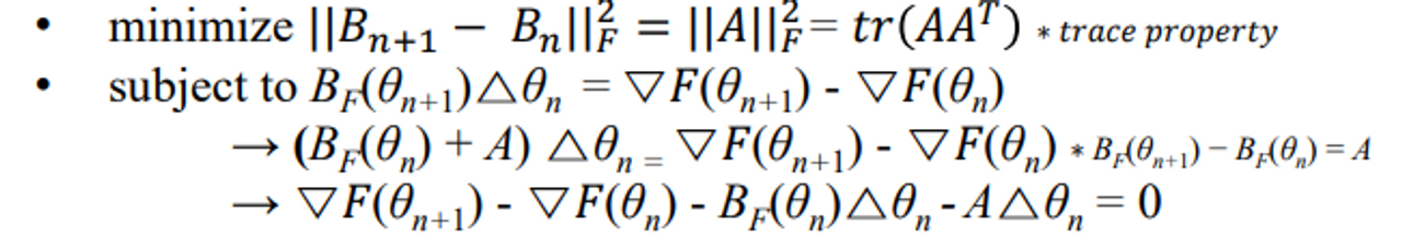
목표는 다음과 같다
→ 수식을 통해 $H(θ_n) = H(θ_{n+1})$ 거의 같게 만드는 문제를 풀면 업데이트 함수로 진화할 수 있다는 것이다.

This can be achieved by minimizing the Frobenius norm of the difference between Bn+1 and Bn, subject to the secant equation constraint:
- 지금 하고자 하는 것은 업데이트 전과 후가 비슷하도록 만드는 것이다.
- secant 성질을 만족해야한다 그래서 (subject to ~) 문장을 조건으로 건다.
  
  ⇒ 무언가 minimize 하는데 constraint가 걸려있다 => Lagrange 등장!

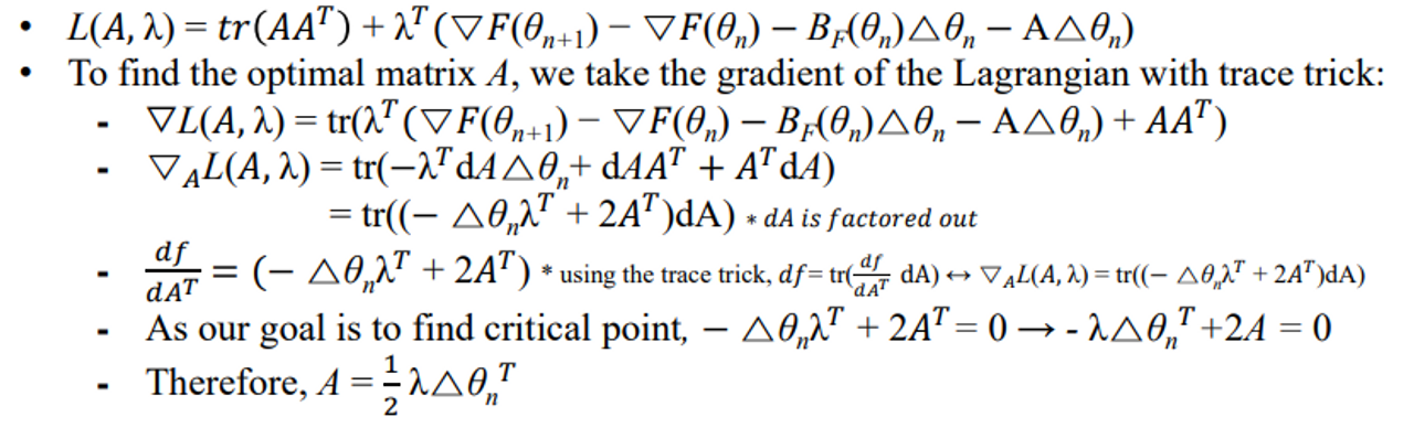
Here, Lagrange multiplier λ is used to form the Lagrangian:
- 그래디언트를 때리는데 람다는 사용하지 않는다. 왜냐면 어처피 0 이기 때문이다.
- A에 대해 편미분을 때리면 아래와 같은 식이 나오는데…
- 정리하면 최종적으로 식이 나온다.