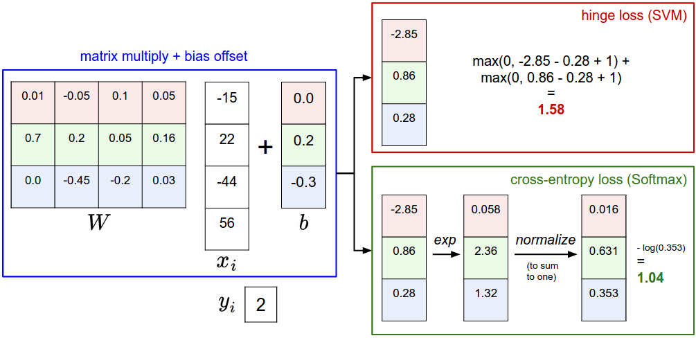
softmax vs SVM
softmax 분류 구현하기
train, validation, test, dev case로 나누기
def get_CIFAR10_data(num_training=49000, num_validation=1000, num_test=1000, num_dev=500):
    """
    Load the CIFAR-10 dataset from disk and perform preprocessing to prepare
    it for the linear classifier. These are the same steps as we used for the
    SVM, but condensed to a single function.
    """
    # Load the raw CIFAR-10 data
    cifar10_dir = 'cs231n/datasets/cifar-10-batches-py'

    # Cleaning up variables to prevent loading data multiple times (which may cause memory issue)
    try:
       del X_train, y_train
       del X_test, y_test
       print('Clear previously loaded data.')
    except:
       pass

    X_train, y_train, X_test, y_test = load_CIFAR10(cifar10_dir)

    # subsample the data
    mask = list(range(num_training, num_training + num_validation))
    X_val = X_train[mask]
    y_val = y_train[mask]
    mask = list(range(num_training))
    X_train = X_train[mask]
    y_train = y_train[mask]
    mask = list(range(num_test))
    X_test = X_test[mask]
    y_test = y_test[mask]
    mask = np.random.choice(num_training, num_dev, replace=False)
    X_dev = X_train[mask]
    y_dev = y_train[mask]

    # Preprocessing: reshape the image data into rows
    X_train = np.reshape(X_train, (X_train.shape[0], -1))
    X_val = np.reshape(X_val, (X_val.shape[0], -1))
    X_test = np.reshape(X_test, (X_test.shape[0], -1))
    X_dev = np.reshape(X_dev, (X_dev.shape[0], -1))

    # Normalize the data: subtract the mean image
    mean_image = np.mean(X_train, axis = 0)
    X_train -= mean_image
    X_val -= mean_image
    X_test -= mean_image
    X_dev -= mean_image

    # add bias dimension and transform into columns
    X_train = np.hstack([X_train, np.ones((X_train.shape[0], 1))])
    X_val = np.hstack([X_val, np.ones((X_val.shape[0], 1))])
    X_test = np.hstack([X_test, np.ones((X_test.shape[0], 1))])
    X_dev = np.hstack([X_dev, np.ones((X_dev.shape[0], 1))])

    return X_train, y_train, X_val, y_val, X_test, y_test, X_dev, y_dev


# Invoke the above function to get our data.
X_train, y_train, X_val, y_val, X_test, y_test, X_dev, y_dev = get_CIFAR10_data()
print('Train data shape: ', X_train.shape)
print('Train labels shape: ', y_train.shape)
print('Validation data shape: ', X_val.shape)
print('Validation labels shape: ', y_val.shape)
print('Test data shape: ', X_test.shape)
print('Test labels shape: ', y_test.shape)
print('dev data shape: ', X_dev.shape)
print('dev labels shape: ', y_dev.shape)
Train data shape: (49000, 3073)
Train labels shape: (49000,)
Validation data shape: (1000, 3073)
Validation labels shape: (1000,)
Test data shape: (1000, 3073)
Test labels shape: (1000,)
dev data shape: (500, 3073)
dev labels shape: (500,)
# First implement the naive softmax loss function with nested loops.
# Open the file cs231n/classifiers/softmax.py and implement the
# softmax_loss_naive function.

from cs231n.classifiers.softmax import softmax_loss_naive
import time

# Generate a random softmax weight matrix and use it to compute the loss.
W = np.random.randn(3073, 10) * 0.0001 # 평균 0, 표준편차 1의 정규분포 난수를 (3073, 10) 생성
loss, grad = softmax_loss_naive(W, X_dev, y_dev, 0.0)

# As a rough sanity check, our loss should be something close to -log(0.1).
# loss 가 -log(0.1)에 가까울 것
# 가중치 행렬이 0에 가까운 난수로 초기화될 때, 점수는 모두 대략 동일하다.

print('loss: %f' % loss)
print('sanity check: %f' % (-np.log(0.1)))
softmax_loss_native 함수 구현하기
def softmax_loss_naive(W, X, y, reg):
    """
    Softmax loss function, naive implementation (with loops)

    Inputs have dimension D, there are C classes, and we operate on minibatches
    of N examples.

    Inputs:
    - W: A numpy array of shape (D, C) containing weights.
    - X: A numpy array of shape (N, D) containing a minibatch of data.
    - y: A numpy array of shape (N,) containing training labels; y[i] = c means
      that X[i] has label c, where 0 <= c < C.
    - reg: (float) regularization strength

    Returns a tuple of:
    - loss as single float
    - gradient with respect to weights W; an array of same shape as W
    """
    # Initialize the loss and gradient to zero.
    loss = 0.0
    dW = np.zeros_like(W)

    #############################################################################
    # TODO: Compute the softmax loss and its gradient using explicit loops.     #
    # Store the loss in loss and the gradient in dW. If you are not careful     #
    # here, it is easy to run into numeric instability. Don't forget the        #
    # regularization!                                                           #
    #############################################################################
    # *****START OF YOUR CODE (DO NOT DELETE/MODIFY THIS LINE)*****

    num_train = X.shape[0] # X_dev.shape[0] = 500 -> 500개의 데이터
    num_classes = W.shape[1] # X_dev.shape[1] = 10 -> 10개의 클래스
    for i in range(num_train): # 500번 반복
        scores = X[i].dot(W) # (i, 3073) * (3073, 10) = (i, 10)
        scores -= np.max(scores) # overflow 방지
        correct_class_score = scores[y[i]] # 정답 클래스의 점수
        exp_sum = np.sum(np.exp(scores)) # 모든 클래스의 점수의 합
        loss += -correct_class_score + np.log(exp_sum) # loss 계산, 500개의 loss의 합
        for j in range(num_classes): # 10번 반복
            dW[:, j] += X[i] * np.exp(scores[j]) / exp_sum # gradient 계산
        dW[:, y[i]] -= X[i] # 정답 클래스의 gradient 계산

    # 평균 loss, gradient 계산
    loss /= num_train # 평균 loss 계산, loss = -log(softmax)
    # softmax의 loss는 -log(softmax)인 이유, https://www.youtube.com/watch?v=OoUX-nOEjG0

    # 아래 loss는 작동하지 않음
    loss += reg * np.sum(W * W) # regularization loss 계산, loss = -log(softmax) + reg * W^2
    # loss가 -log(0.1) = 2.3 정도로 나오는데, 이는 정답 클래스의 점수가 0.1이라는 뜻이다.
    # 이는 softmax 함수의 결과가 0.1이라는 뜻이다.

    dW /= num_train # 평균 gradient 계산
    dW += 2 * reg * W # regularization gradient 계산
    pass

    # *****END OF YOUR CODE (DO NOT DELETE/MODIFY THIS LINE)*****

    return loss, dW
loss가 -log(0.1)과 유사하다.
loss: 2.322386
sanity check: 2.302585
softmax 손실함수 실행
# Complete the implementation of softmax_loss_naive and implement a (naive)
# version of the gradient that uses nested loops.
loss, grad = softmax_loss_naive(W, X_dev, y_dev, 0.0)

# As we did for the SVM, use numeric gradient checking as a debugging tool.
# The numeric gradient should be close to the analytic gradient.
from cs231n.gradient_check import grad_check_sparse
f = lambda w: softmax_loss_naive(w, X_dev, y_dev, 0.0)[0]
grad_numerical = grad_check_sparse(f, W, grad, 10)

# similar to SVM case, do another gradient check with regularization
loss, grad = softmax_loss_naive(W, X_dev, y_dev, 5e1)
f = lambda w: softmax_loss_naive(w, X_dev, y_dev, 5e1)[0]
numerical: 0.385269 analytic: 0.385269, relative error: 1.332712e-08
numerical: -2.685121 analytic: -2.685121, relative error: 5.910057e-09
numerical: -0.484391 analytic: -0.484391, relative error: 3.695873e-08
numerical: 2.634291 analytic: 2.634291, relative error: 1.514669e-08
numerical: 2.389521 analytic: 2.389521, relative error: 2.969521e-08
numerical: -0.096752 analytic: -0.096752, relative error: 4.204243e-07
numerical: -1.450224 analytic: -1.450224, relative error: 7.030728e-09
numerical: -1.867091 analytic: -1.867091, relative error: 3.841828e-08
numerical: 4.281678 analytic: 4.281678, relative error: 2.005822e-08
numerical: 0.842029 analytic: 0.842028, relative error: 5.663032e-08
numerical: -1.370057 analytic: -1.370057, relative error: 7.795995e-09
numerical: 0.616715 analytic: 0.616715, relative error: 1.019285e-07
numerical: -2.465819 analytic: -2.465819, relative error: 8.009716e-09
numerical: -0.643678 analytic: -0.643678, relative error: 1.159443e-08
numerical: 5.270430 analytic: 5.270430, relative error: 1.436576e-08
numerical: -0.946898 analytic: -0.946898, relative error: 9.727613e-09
numerical: 2.138761 analytic: 2.138761, relative error: 1.323439e-08
numerical: 0.657479 analytic: 0.657479, relative error: 5.639085e-08
numerical: 2.498252 analytic: 2.498251, relative error: 3.748569e-08
numerical: 0.421892 analytic: 0.421892, relative error: 1.572079e-08
vecorized 버전으로 softmax 손실함수 구현하기
def softmax_loss_vectorized(W, X, y, reg):
    """
    Softmax loss function, vectorized version.

    Inputs and outputs are the same as softmax_loss_naive.
    """
    # Initialize the loss and gradient to zero.
    loss = 0.0
    dW = np.zeros_like(W)

    #############################################################################
    # TODO: Compute the softmax loss and its gradient using no explicit loops.  #
    # Store the loss in loss and the gradient in dW. If you are not careful     #
    # here, it is easy to run into numeric instability. Don't forget the        #
    # regularization!                                                           #
    #############################################################################
    # *****START OF YOUR CODE (DO NOT DELETE/MODIFY THIS LINE)*****

    num_train = X.shape[0] # X_dev.shape[0] = 500 -> 500개의 데이터
    scores = X.dot(W) # (500, 3073) * (3073, 10) = (500, 10)
    scores -= np.max(scores, axis=1, keepdims=True) # overflow 방지
    correct_class_score = scores[np.arange(num_train), y] # 정답 클래스의 점수
    exp_sum = np.sum(np.exp(scores), axis=1) # 모든 클래스의 점수의 합
    loss = np.sum(-correct_class_score + np.log(exp_sum)) # loss 계산
    loss /= num_train # 평균 loss 계산
    loss += reg * np.sum(W * W) # regularization loss 계산
    softmax = np.exp(scores) / exp_sum.reshape(-1, 1) # softmax 계산
    softmax[np.arange(num_train), y] -= 1 # 정답 클래스의 gradient 계산
    dW = X.T.dot(softmax) # gradient 계산
    dW /= num_train # 평균 gradient 계산
    dW += 2 * reg * W # regularization gradient 계산
    pass

    # *****END OF YOUR CODE (DO NOT DELETE/MODIFY THIS LINE)*****

    return loss, dW
두 버전의 속도 비교하기
# Now that we have a naive implementation of the softmax loss function and its gradient,
# implement a vectorized version in softmax_loss_vectorized.
# The two versions should compute the same results, but the vectorized version should be
# much faster.
tic = time.time()
loss_naive, grad_naive = softmax_loss_naive(W, X_dev, y_dev, 0.000005)
toc = time.time()
print('naive loss: %e computed in %fs' % (loss_naive, toc - tic))

from cs231n.classifiers.softmax import softmax_loss_vectorized
tic = time.time()
loss_vectorized, grad_vectorized = softmax_loss_vectorized(W, X_dev, y_dev, 0.000005)
toc = time.time()
print('vectorized loss: %e computed in %fs' % (loss_vectorized, toc - tic))

# As we did for the SVM, we use the Frobenius norm to compare the two versions
# of the gradient.
grad_difference = np.linalg.norm(grad_naive - grad_vectorized, ord='fro')
print('Loss difference: %f' % np.abs(loss_naive - loss_vectorized))
print('Gradient difference: %f' % grad_difference)
vectorized loss가 더 빠른 것을 알 수 있다.
naive loss: 2.322386e+00 computed in 0.071012s
vectorized loss: 2.322386e+00 computed in 0.004780s
Loss difference: 0.000000
Gradient difference: 0.000000
검증세트로 튜닝하기
# Use the validation set to tune hyperparameters (regularization strength and
# learning rate). You should experiment with different ranges for the learning
# rates and regularization strengths; if you are careful you should be able to
# get a classification accuracy of over 0.35 on the validation set.

from cs231n.classifiers import Softmax
results = {}
best_val = -1
best_softmax = None

################################################################################
# TODO:                                                                        #
# Use the validation set to set the learning rate and regularization strength. #
# This should be identical to the validation that you did for the SVM; save    #
# the best trained softmax classifer in best_softmax.                          #
################################################################################

# Provided as a reference. You may or may not want to change these hyperparameters
learning_rates = [1e-7, 5e-7]
regularization_strengths = [2.5e4, 5e4]

# *****START OF YOUR CODE (DO NOT DELETE/MODIFY THIS LINE)*****
for lr in learning_rates:
    for reg in regularization_strengths:
        sfm = Softmax()
        loss_history = sfm.train(X_train, y_train, learning_rate=lr, reg=reg, num_iters=1500, verbose=False)
        y_train_pred = sfm.predict(X_train) # 예측값
        train_accuracy = np.mean(y_train == y_train_pred) # 정확도
        y_val_pred = sfm.predict(X_val) # val에 대한 예측값
        val_accuracy = np.mean(y_val == y_val_pred) # val에 대한 정확도
        results[(lr,reg)] = (train_accuracy, val_accuracy) # 결과 정리
        if val_accuracy > best_val:
            best_val = val_accuracy
            best_softmax = sfm
pass

# *****END OF YOUR CODE (DO NOT DELETE/MODIFY THIS LINE)*****

# Print out results.
for lr, reg in sorted(results):
    train_accuracy, val_accuracy = results[(lr, reg)]
    print('lr %e reg %e train accuracy: %f val accuracy: %f' % (
                lr, reg, train_accuracy, val_accuracy))

print('best validation accuracy achieved during cross-validation: %f' % best_val)
lr 1.000000e-07 reg 2.500000e+04 train accuracy: 0.328469 val accuracy: 0.347000
lr 1.000000e-07 reg 5.000000e+04 train accuracy: 0.305939 val accuracy: 0.319000
lr 5.000000e-07 reg 2.500000e+04 train accuracy: 0.331592 val accuracy: 0.354000
lr 5.000000e-07 reg 5.000000e+04 train accuracy: 0.304122 val accuracy: 0.316000
best validation accuracy achieved during cross-validation: 0.354000
SVM 분류기의 경우, 손실이 마진에 기초하고 손실 함수는 마진 아래의 값에 0을 할당하기 때문에 실질적으로 손실이 없는 것이 가능하다. Softmax Classifier의 경우, 이는 사실이 아니며, 새 데이터 포인트에 대해 손실이 전혀 발생하지 않습니다. (SVM은 로컬 목표인 반면 Softmax Classifier는 그렇지 않습니다.)
# evaluate on test set
# Evaluate the best softmax on test set
y_test_pred = best_softmax.predict(X_test)
test_accuracy = np.mean(y_test == y_test_pred)
print('softmax on raw pixels final test set accuracy: %f' % (test_accuracy, ))
softmax on raw pixels final test set accuracy: 0.354000
데이터 시각화
# Visualize the learned weights for each class
w = best_softmax.W[:-1,:] # strip out the bias
w = w.reshape(32, 32, 3, 10)

w_min, w_max = np.min(w), np.max(w)

classes = ['plane', 'car', 'bird', 'cat', 'deer', 'dog', 'frog', 'horse', 'ship', 'truck']
for i in range(10):
    plt.subplot(2, 5, i + 1)

    # Rescale the weights to be between 0 and 255
    wimg = 255.0 * (w[:, :, :, i].squeeze() - w_min) / (w_max - w_min)
    plt.imshow(wimg.astype('uint8'))
    plt.axis('off')
    plt.title(classes[i])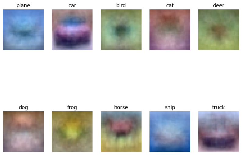
kNN 분류기와 달리 이 매개 변수 접근법의 장점은 매개 변수를 학습하면 훈련 데이터를 폐기할 수 있다는 것이다. 또한, 새로운 테스트 이미지에 대한 예측은 모든 단일 훈련 예제와 완전한 비교가 아니라 W를 사용한 단일 행렬 곱셈이 필요하기 때문에 빠르다.
