
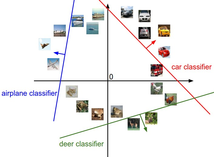
Linear Classification
cifar10 데이터 불러오는 과정은 생략
Split the data sets
# Split the data into train, val, and test sets. In addition we will
# create a small development set as a subset of the training data;
# we can use this for development so our code runs faster.
num_training = 49000
num_validation = 1000
num_test = 1000
num_dev = 500

# Our validation set will be num_validation points from the original
# training set.
mask = range(num_training, num_training + num_validation)
X_val = X_train[mask]
y_val = y_train[mask]

# Our training set will be the first num_train points from the original
# training set.
mask = range(num_training)
X_train = X_train[mask]
y_train = y_train[mask]

# We will also make a development set, which is a small subset of
# the training set.
mask = np.random.choice(num_training, num_dev, replace=False)
X_dev = X_train[mask]
y_dev = y_train[mask]

# We use the first num_test points of the original test set as our
# test set.
mask = range(num_test)
X_test = X_test[mask]
y_test = y_test[mask]

print('Train data shape: ', X_train.shape)
print('Train labels shape: ', y_train.shape)
print('Validation data shape: ', X_val.shape)
print('Validation labels shape: ', y_val.shape)
print('Test data shape: ', X_test.shape)
데이터 형식 변환(reshape)
# Preprocessing: reshape the image data into rows
X_train = np.reshape(X_train, (X_train.shape[0], -1))
X_val = np.reshape(X_val, (X_val.shape[0], -1))
X_test = np.reshape(X_test, (X_test.shape[0], -1))
X_dev = np.reshape(X_dev, (X_dev.shape[0], -1))

# As a sanity check, print out the shapes of the data
print('Training data shape: ', X_train.shape)
print('Validation data shape: ', X_val.shape)
print('Test data shape: ', X_test.shape)
print('dev data shape: ', X_dev.shape)
Training data shape: (49000, 3072)
Validation data shape: (1000, 3072)
Test data shape: (1000, 3072)
dev data shape: (500, 3072)
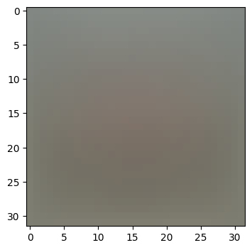
이미지 평균 출력하기
# Preprocessing: subtract the mean image
# first: compute the image mean based on the training data
mean_image = np.mean(X_train, axis=0)
print(mean_image[:10]) # print a few of the elements
plt.figure(figsize=(4,4))
plt.imshow(mean_image.reshape((32,32,3)).astype('uint8')) # visualize the mean image
plt.show()

# second: subtract the mean image from train and test data
X_train -= mean_image
X_val -= mean_image
X_test -= mean_image
X_dev -= mean_image

# third: append the bias dimension of ones (i.e. bias trick) so that our SVM
# only has to worry about optimizing a single weight matrix W.
X_train = np.hstack([X_train, np.ones((X_train.shape[0], 1))])
X_val = np.hstack([X_val, np.ones((X_val.shape[0], 1))])
X_test = np.hstack([X_test, np.ones((X_test.shape[0], 1))])
X_dev = np.hstack([X_dev, np.ones((X_dev.shape[0], 1))])

print(X_train.shape, X_val.shape, X_test.shape, X_dev.shape)
요상한 이미지가 나온다(이미지의 데이터의 단순 평균)
[130.64189796 135.98173469 132.47391837 130.05569388 135.34804082
131.75402041 130.96055102 136.14328571 132.47636735 131.48467347]
svm_loss_naive 함수 구현
def svm_loss_naive(W, X, y, reg):
   """
   Structured SVM loss function, naive implementation (with loops).

   Inputs have dimension D, there are C classes, and we operate on minibatches
   of N examples.

   Inputs:
   - W: A numpy array of shape (D, C) containing weights.
   - X: A numpy array of shape (N, D) containing a minibatch of data.
   - y: A numpy array of shape (N,) containing training labels; y[i] = c means
     that X[i] has label c, where 0 <= c < C.
   - reg: (float) regularization strength

   Returns a tuple of:
   - loss as single float
   - gradient with respect to weights W; an array of same shape as W
   """
   dW = np.zeros(W.shape)  # initialize the gradient as zero

   # compute the loss and the gradient
   num_classes = W.shape[1]
   num_train = X.shape[0]
   loss = 0.0
   for i in range(num_train):
       scores = X[i].dot(W)
       correct_class_score = scores[y[i]]
       for j in range(num_classes):
           if j == y[i]:
               continue
           margin = scores[j] - correct_class_score + 1  # note delta = 1
           if margin > 0:
               loss += margin

   # Right now the loss is a sum over all training examples, but we want it
   # to be an average instead so we divide by num_train.
   loss /= num_train

   # Add regularization to the loss.
   loss += reg * np.sum(W * W)

   #############################################################################
   # TODO:                                                                     #
   # Compute the gradient of the loss function and store it dW.                #
   # Rather that first computing the loss and then computing the derivative,   #
   # it may be simpler to compute the derivative at the same time that the     #
   # loss is being computed. As a result you may need to modify some of the    #
   # code above to compute the gradient.                                       #
   #############################################################################
   # *****START OF YOUR CODE (DO NOT DELETE/MODIFY THIS LINE)*****

   # dW는 W의 shape과 같은 크기의 0으로 채워진 행렬이다.
   dW += 2 * reg * W # regularization gradient
   pass

   # *****END OF YOUR CODE (DO NOT DELETE/MODIFY THIS LINE)*****

   return loss, dW
테스트
# Evaluate the naive implementation of the loss we provided for you:
from cs231n.classifiers.linear_svm import svm_loss_naive
import time

# generate a random SVM weight matrix of small numbers
W = np.random.randn(3073, 10) * 0.0001

loss, grad = svm_loss_naive(W, X_dev, y_dev, 0.000005)
print('loss: %f' % (loss, ))
loss: 8.597039
# Once you've implemented the gradient, recompute it with the code below
# and gradient check it with the function we provided for you

# Compute the loss and its gradient at W.
loss, grad = svm_loss_naive(W, X_dev, y_dev, 0.0)

# Numerically compute the gradient along several randomly chosen dimensions, and
# compare them with your analytically computed gradient. The numbers should match
# almost exactly along all dimensions.
from cs231n.gradient_check import grad_check_sparse
f = lambda w: svm_loss_naive(w, X_dev, y_dev, 0.0)[0]
grad_numerical = grad_check_sparse(f, W, grad)

# do the gradient check once again with regularization turned on
# you didn't forget the regularization gradient did you?
loss, grad = svm_loss_naive(W, X_dev, y_dev, 5e1)
f = lambda w: svm_loss_naive(w, X_dev, y_dev, 5e1)[0]
grad_numerical = grad_check_sparse(f, W, grad)
Inline Question 1
It is possible that once in a while a dimension in the gradcheck will not match exactly. What could such a discrepancy be caused by? Is it a reason for concern? What is a simple example in one dimension where a gradient check could fail? How would change the margin affect of the frequency of this happening? Hint: the SVM loss function is not strictly speaking differentiable
수치 근사값을 사용(?) 하기 때문에 오차가 발생할 수 있다.
Increasing the margin would make a mismatch in the numerical and analytical answers more unlikely
svm_loss_vertorized 함수 구현
def svm_loss_vectorized(W, X, y, reg):
    """
    Structured SVM loss function, vectorized implementation.

    Inputs and outputs are the same as svm_loss_naive.
    """
    loss = 0.0
    dW = np.zeros(W.shape)  # initialize the gradient as zero

    #############################################################################
    # TODO:                                                                     #
    # Implement a vectorized version of the structured SVM loss, storing the    #
    # result in loss.                                                           #
    #############################################################################
    # *****START OF YOUR CODE (DO NOT DELETE/MODIFY THIS LINE)*****

    scores = X @ W
    x = np.arange(X.shape[0])
    margins = np.maximum(0, (scores.T - scores[x, y]).T + 1)
    margins[x, y] = 0
    indicator = (margins > 0).astype(float)
    indicator_sum = np.sum(indicator, axis=1)
    indicator[x, y] -= indicator_sum[x]
    loss = np.sum(margins) / X.shape[0] + reg * np.sum(W * W)
    pass

    # *****END OF YOUR CODE (DO NOT DELETE/MODIFY THIS LINE)*****

    #############################################################################
    # TODO:                                                                     #
    # Implement a vectorized version of the gradient for the structured SVM     #
    # loss, storing the result in dW.                                           #
    #                                                                           #
    # Hint: Instead of computing the gradient from scratch, it may be easier    #
    # to reuse some of the intermediate values that you used to compute the     #
    # loss.                                                                     #
    #############################################################################
    # *****START OF YOUR CODE (DO NOT DELETE/MODIFY THIS LINE)*****

    dW += (X.T @ indicator) / X.shape[0]
    dW += 2 * reg * W

    pass

    # *****END OF YOUR CODE (DO NOT DELETE/MODIFY THIS LINE)*****

    return loss, dW
Navie loss와 Vectorized loss가 같아졌다.
Naive loss: 9.133378e+00 computed in 0.025214s
Vectorized loss: 9.133378e+00 computed in 0.037167s
difference: 0.000000
각각 시간을 비교한다.
# Next implement the function svm_loss_vectorized; for now only compute the loss;
# we will implement the gradient in a moment.
tic = time.time()
loss_naive, grad_naive = svm_loss_naive(W, X_dev, y_dev, 0.000005)
toc = time.time()
print('Naive loss: %e computed in %fs' % (loss_naive, toc - tic))

from cs231n.classifiers.linear_svm import svm_loss_vectorized
tic = time.time()
loss_vectorized, _ = svm_loss_vectorized(W, X_dev, y_dev, 0.000005)
toc = time.time()
print('Vectorized loss: %e computed in %fs' % (loss_vectorized, toc - tic))

# The losses should match but your vectorized implementation should be much faster.
print('difference: %f' % (loss_naive - loss_vectorized))
Vectorized loss가 더 빠른 것을 알 수 있다.
Naive loss: 8.929968e+00 computed in 0.015665s
Vectorized loss: 8.929968e+00 computed in 0.006835s
difference: 0.000000
확률적 경사 하강법
# In the file linear_classifier.py, implement SGD in the function
# LinearClassifier.train() and then run it with the code below.
from cs231n.classifiers import LinearSVM
svm = LinearSVM()
tic = time.time()
loss_hist = svm.train(X_train, y_train, learning_rate=1e-7, reg=2.5e4,
                      num_iters=1500, verbose=True)
toc = time.time()
print('That took %fs' % (toc - tic))
iteration 0 / 1500: loss 778.844646
iteration 100 / 1500: loss 283.565720
iteration 200 / 1500: loss 106.175843
iteration 300 / 1500: loss 42.317204
iteration 400 / 1500: loss 19.121094
iteration 500 / 1500: loss 10.839462
iteration 600 / 1500: loss 7.356074
iteration 700 / 1500: loss 7.007573
iteration 800 / 1500: loss 5.441904
iteration 900 / 1500: loss 5.200329
iteration 1000 / 1500: loss 5.651302
iteration 1100 / 1500: loss 5.154519
iteration 1200 / 1500: loss 6.107881
iteration 1300 / 1500: loss 5.800412
iteration 1400 / 1500: loss 5.649598
That took 6.484614s
시각화
# A useful debugging strategy is to plot the loss as a function of
# iteration number:
plt.plot(loss_hist)
plt.xlabel('Iteration number')
plt.ylabel('Loss value')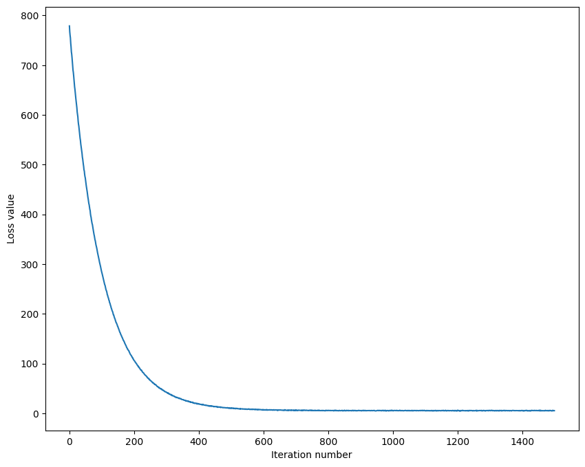
정확도 비교
# Write the LinearSVM.predict function and evaluate the performance on both the
# training and validation set
y_train_pred = svm.predict(X_train)
print('training accuracy: %f' % (np.mean(y_train == y_train_pred), ))
y_val_pred = svm.predict(X_val)
print('validation accuracy: %f' % (np.mean(y_val == y_val_pred), ))
training accuracy: 0.368163
validation accuracy: 0.384000
검증 세트를 통한 튜닝
# Use the validation set to tune hyperparameters (regularization strength and
# learning rate). You should experiment with different ranges for the learning
# rates and regularization strengths; if you are careful you should be able to
# get a classification accuracy of about 0.39 (> 0.385) on the validation set.

# Note: you may see runtime/overflow warnings during hyper-parameter search.
# This may be caused by extreme values, and is not a bug.

# results is dictionary mapping tuples of the form
# (learning_rate, regularization_strength) to tuples of the form
# (training_accuracy, validation_accuracy). The accuracy is simply the fraction
# of data points that are correctly classified.
results = {}
best_val = -1   # The highest validation accuracy that we have seen so far.
best_svm = None # The LinearSVM object that achieved the highest validation rate.

################################################################################
# TODO:                                                                        #
# Write code that chooses the best hyperparameters by tuning on the validation #
# set. For each combination of hyperparameters, train a linear SVM on the      #
# training set, compute its accuracy on the training and validation sets, and  #
# store these numbers in the results dictionary. In addition, store the best   #
# validation accuracy in best_val and the LinearSVM object that achieves this  #
# accuracy in best_svm.                                                        #
#                                                                              #
# Hint: You should use a small value for num_iters as you develop your         #
# validation code so that the SVMs don't take much time to train; once you are #
# confident that your validation code works, you should rerun the validation   #
# code with a larger value for num_iters.                                      #
################################################################################

# Provided as a reference. You may or may not want to change these hyperparameters
learning_rates = [5e-8, 1e-7, 5e-7, 1e-6]
regularization_strengths = [5e3, 1e4, 2.5e4, 5e4]

# *****START OF YOUR CODE (DO NOT DELETE/MODIFY THIS LINE)*****
for lr in learning_rates:
  for reg in regularization_strengths:
    svm = LinearSVM()
    svm.train(X_train, y_train, lr, reg,
                      num_iters=1500, verbose=True)
    y_train_pred = svm.predict(X_train)
    y_train_accuracy = np.mean(y_train_pred == y_train)
    y_val_pred = svm.predict(X_val)
    y_val_accuracy = np.mean(y_val_pred == y_val)
    results[(lr,reg)] = (y_train_accuracy, y_val_accuracy)
    if(y_val_accuracy > best_val):
      best_val = y_val_accuracy
      best_svm = svm
pass

# *****END OF YOUR CODE (DO NOT DELETE/MODIFY THIS LINE)*****

# Print out results.
for lr, reg in sorted(results):
    train_accuracy, val_accuracy = results[(lr, reg)]
    print('lr %e reg %e train accuracy: %f val accuracy: %f' % (
                lr, reg, train_accuracy, val_accuracy))

print('best validation accuracy achieved during cross-validation: %f' % best_val)
lr 5.000000e-08 reg 5.000000e+03 train accuracy: 0.323714 val accuracy: 0.323000
lr 5.000000e-08 reg 1.000000e+04 train accuracy: 0.358020 val accuracy: 0.376000
lr 5.000000e-08 reg 2.500000e+04 train accuracy: 0.370816 val accuracy: 0.389000
lr 5.000000e-08 reg 5.000000e+04 train accuracy: 0.362857 val accuracy: 0.377000
lr 1.000000e-07 reg 5.000000e+03 train accuracy: 0.373531 val accuracy: 0.379000
lr 1.000000e-07 reg 1.000000e+04 train accuracy: 0.382306 val accuracy: 0.383000
lr 1.000000e-07 reg 2.500000e+04 train accuracy: 0.360714 val accuracy: 0.367000
lr 1.000000e-07 reg 5.000000e+04 train accuracy: 0.360449 val accuracy: 0.356000
lr 5.000000e-07 reg 5.000000e+03 train accuracy: 0.369857 val accuracy: 0.380000
lr 5.000000e-07 reg 1.000000e+04 train accuracy: 0.359122 val accuracy: 0.369000
lr 5.000000e-07 reg 2.500000e+04 train accuracy: 0.341449 val accuracy: 0.328000
lr 5.000000e-07 reg 5.000000e+04 train accuracy: 0.326327 val accuracy: 0.344000
lr 1.000000e-06 reg 5.000000e+03 train accuracy: 0.357551 val accuracy: 0.362000
lr 1.000000e-06 reg 1.000000e+04 train accuracy: 0.317143 val accuracy: 0.332000
lr 1.000000e-06 reg 2.500000e+04 train accuracy: 0.284306 val accuracy: 0.309000
lr 1.000000e-06 reg 5.000000e+04 train accuracy: 0.290959 val accuracy: 0.289000
best validation accuracy achieved during cross-validation: 0.389000
시각화
# Visualize the cross-validation results
import math
import pdb

# pdb.set_trace()

x_scatter = [math.log10(x[0]) for x in results]
y_scatter = [math.log10(x[1]) for x in results]

# plot training accuracy
marker_size = 100
colors = [results[x][0] for x in results]
plt.subplot(2, 1, 1)
plt.tight_layout(pad=3)
plt.scatter(x_scatter, y_scatter, marker_size, c=colors, cmap=plt.cm.coolwarm)
plt.colorbar()
plt.xlabel('log learning rate')
plt.ylabel('log regularization strength')
plt.title('CIFAR-10 training accuracy')

# plot validation accuracy
colors = [results[x][1] for x in results] # default size of markers is 20
plt.subplot(2, 1, 2)
plt.scatter(x_scatter, y_scatter, marker_size, c=colors, cmap=plt.cm.coolwarm)
plt.colorbar()
plt.xlabel('log learning rate')
plt.ylabel('log regularization strength')
plt.title('CIFAR-10 validation accuracy')
plt.show()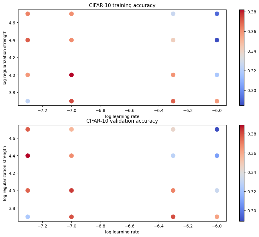
최적의 정확도
# Evaluate the best svm on test set
y_test_pred = best_svm.predict(X_test)
test_accuracy = np.mean(y_test == y_test_pred)
print('linear SVM on raw pixels final test set accuracy: %f' % test_accuracy)
linear SVM on raw pixels final test set accuracy: 0.368000
각 클래스의 시각화
# Visualize the learned weights for each class.
# Depending on your choice of learning rate and regularization strength, these may
# or may not be nice to look at.
w = best_svm.W[:-1,:] # strip out the bias
w = w.reshape(32, 32, 3, 10)
w_min, w_max = np.min(w), np.max(w)
classes = ['plane', 'car', 'bird', 'cat', 'deer', 'dog', 'frog', 'horse', 'ship', 'truck']
for i in range(10):
    plt.subplot(2, 5, i + 1)

    # Rescale the weights to be between 0 and 255
    wimg = 255.0 * (w[:, :, :, i].squeeze() - w_min) / (w_max - w_min)
    plt.imshow(wimg.astype('uint8'))
    plt.axis('off')
    plt.title(classes[i])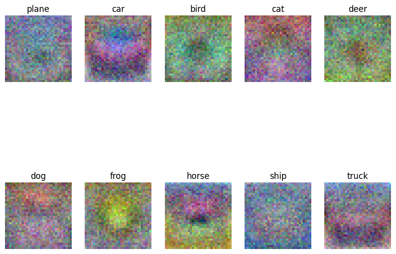
Describe what your visualized SVM weights look like, and offer a brief explanation for why they look the way they do.
템플릿과 유사한 이미지는 높은 점수를 할당받고 아닌경우는 낮은 점수를 할당받는다.!
