활성홯마수(중산층)
초기: stepfunction
sigmoid (경사하강법 진행시) 미분을 해야하는 데 기울기가 필요
relu mlp 학습시 층이 깊어지면서 기울시소실 현상이 발생 -> 오차가 줄어보이는 문제점!
경사하강법
경사하강법 (GD)
전체딩터를 이용해 업데이트
확률적 견사하강법 (SGD)
확률적으로 선택된 " 일부 데이터 를 이용하여 업데이트
단점: 비효율적인 학습
모멘텀 momentum
관성이라는 원리를 도입라여 이전 batch_size을 방영
기본배치사이즈: 32
네스테로프 모멘텀 (NAG/)
이후 배치를 반영 -> 불필요한 이동을 줄일 수 있다
에이다그래드 (AdaGrad)
학습률 (보푹) 감소방법을 적용 , 처음엔느 크게 학습하나가 조금씩 작세 학습한는 방법으로 빠르고 정확한 학습니 가능
아담 (adam)
학습방향, 보푹을 모두 고려하려 적절하세 사용
다양한 활성화함수 와 경사하겅법에 떠른 성능비교
1. sigmoid + SGD
2. relu + SGD
3. relu + Adam
Library 불러오기
import numpy as np
import pandas as pd
import matplotlib.pyplot as plt
from tensorflow.keras import Sequential
from tensorflow.keras.layers import Dense, InputLayer, Flatten
# optimizer 불러오기 (최적화함수 틀래스 불러와사 사용해보기
from tensorflow.keras.optimizers import SGD, Adam
데이터 불로오기 (4개의 변수에 담기!
x_train, y_train, x_test, y_test)
from tensorflow.keras.datasets import mnist
(x_train, y_train),(x_test, y_test) = mnist.load_data()
print(x_train.shape, y_train.shape)
print(x_test.shape, y_test.shape)
1. 모델링 설계 (model 1, model 2, model 3)
중간층 (총 5개위 층, units = 64,128,256,128,64)
model1 = Sequential()
model1.add (InputLayer(input_shape=(28,28)))
model1.add(Flatten())
model1.add(Dense(units = 64, activation ='sigmoid'))
model1.add(Dense(units = 128, activation ='sigmoid'))
model1.add(Dense(units = 256, activation ='sigmoid'))
model1.add(Dense(units = 128, activation ='sigmoid'))
model1.add(Dense(units = 64, activation ='sigmoid'))
model1.add(Dense(units  =10, activation = 'softmax'))
model2 = Sequential()
model2.add (InputLayer(input_shape=(28,28)))
model2.add(Flatten())
model2.add(Dense(units = 64, activation ='relu'))
model2.add(Dense(units = 128, activation ='relu'))
model2.add(Dense(units = 256, activation ='relu'))
model2.add(Dense(units = 128, activation ='relu'))
model2.add(Dense(units = 64, activation ='relu'))
model2.add(Dense(units =10, activation = 'softmax'))model3 = Sequential()
model3.add (InputLayer(input_shape=(28,28)))
model3.add(Flatten())
model3.add(Dense(units = 64, activation ='relu'))
model3.add(Dense(units = 128, activation ='relu'))
model3.add(Dense(units = 256, activation ='relu'))
model3.add(Dense(units = 128, activation ='relu'))
model3.add(Dense(units = 64, activation ='relu'))
model3.add(Dense(units =10, activation = 'softmax'))2. 학습방법 및 평가방법 설정
model1.compile(loss = 'sparse_categorical_crossentropy',
optimizer = 'SGD', metrics = ['accuracy'])model2.compile(loss = 'sparse_categorical_crossentropy',# SGD 한수의 기본 학습률 0.01>0.001
# 중간층의 활성화함수를 relu로 변경하면서 오차가 줄어들지 않게됨
# 여러가 큰값이 그대로 전달되는 것을 줄여주기 위함
optimizer =SGD(learning_rate = 0.001), metrics = ['accuracy'])model3.compile(loss = 'sparse_categorical_crossentropy',
optimizer = 'Adam', metrics = ['accuracy'])3. 학습 (h1, h2, h3)
h1 = model1.fit(x_train,y_train, validation_split=0.2, epochs = 20)h2 = model2.fit(x_train,y_train, validation_split=0.2, epochs = 20)h3 = model3.fit(x_train,y_train, validation_split=0.2, epochs = 20)4 . 평가
model1.evaluate(x_test, y_test)model2.evaluate(x_test, y_test)model3.evaluate(x_test, y_test)시각화 (3개 모델 한번에 시각화 / 총 6개의 직선 비교)
h1 > accuracy, val_accuracy # h2 accuracy, val_accuracy # h3 accuracy, val_accuracy
plt.figure(figsize= (10,5))
plt.plot(h1.history['accuracy'],label = 'sigmoid+SGD train acc')
plt.plot(h1.history['val_accuracy'], label = 'sigmoid+SGD validation acc')
plt.plot(h2.history['accuracy'],label = 'relu+SGD train acc')
plt.plot(h2.history['val_accuracy'], label = 'relu+SGD validation acc')
plt.plot(h3.history['accuracy'],label = 'relu+adam train acc')
plt.plot(h3.history['val_accuracy'], label = 'relu+adam validation acc')
plt.legend()
plt.show()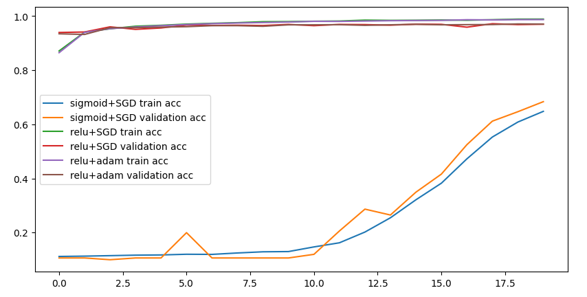
Call backs
모델저장 및 조기학습중단
- 딥러닝 모델 학습시 지정 epochs 가 끝나면 과대적합이 되는 경우가 있는 중간에 일반화된 모델을 저장할 수 맀는 기능이 필요
- 조기락습중단: epochs 를 크게 성장한 경우 일정 획수 이후로는 모델의 성능이 개선되지 않는ㄴ 경우에는 모델 조기학습중단하는 기능이 필요
from tensorflow.keras.callbacks import ModelCheckpoint, EarlyStopping
# 모델 중간저장: Model Checkpoint
# 모델 중간 멈춤: Early Stopping# 모델 저장 객체생성
# 모델을 저장할 경로 설정
model_path = '/content/drive/MyDrive/Colab Notebooks/Deep Learning/data/digit_model/dm_{epoch:02d}_{val_accuracy:0.2f}.hdf5'
mc = ModelCheckpoint(filepath=model_path, # model 저장할 경로
verbose = 1,
# 로그출력: 0 (로그출력 X), 1 (로그 출력 o), 몇번째에 저장되늕지 확인이 가능
save_best_only = True,
# model성능이 최고점을 갱신할때만 저장 (false 매 epoch 마다 저장)
monitor = 'val_accuracy') # 모델의 성능을 확인할 가준
# 일반화 확인을 위하여 val_accuracy 로 선택!
# 모델자장 객체 생성 완료
# 하지만 사용은 아직안한것 > 학습시 객체를 불러와서 사용할것! # 조기학습중단
es = EarlyStopping(monitor = 'val_accuracy', #학습을 중단할 기준겂 설정
verbose = 1 ,# 로그출력
patience = 10) # 모델성능개선을 기다리는 최대 횟수
# 조기학습중단 객체 생성 완료# 1. 모델링 설계 (model 1, model 2, model 3)
# 중간층 (총 5개위 층, units = 64,128,256,128,64)
model1 = Sequential()
model1.add (InputLayer(input_shape=(28,28)))
model1.add(Flatten())
model1.add(Dense(units = 64, activation ='sigmoid'))
model1.add(Dense(units = 128, activation ='sigmoid'))
model1.add(Dense(units = 256, activation ='sigmoid'))
model1.add(Dense(units = 128, activation ='sigmoid'))
model1.add(Dense(units = 64, activation ='sigmoid'))
model1.add(Dense(units =10, activation = 'softmax'))
# 2. 학습방법 및 평가방법 설정
model1.compile(loss = 'sparse_categorical_crossentropy',
optimizer = 'SGD', metrics = ['accuracy'])
# 3. 학습 (h1, h2, h3)
h1 = model1.fit(x_train,y_train, validation_split=0.2, epochs = 1000, callbacks = [mc,es])
# 4 . 평가
model1.evaluate(x_test, y_test)
model 3 학습진행
best_model 이라는 이름으로 모델 지장
1000 번 epoch
best_model = '/content/drive/MyDrive/Colab Notebooks/Deep Learning/data/best_model/bm_{epoch:02d}_{val_accuracy:0.2f}.hdf5'
bm = ModelCheckpoint(filepath=best_model,
verbose = 1,
save_best_only = True,
monitor = 'val_accuracy') es = EarlyStopping(monitor = 'val_accuracy', #학습을 중단할 기준겂 설정
verbose = 1 ,# 로그출력
patience = 10) # 모델성능개선을 기다리는 최대 횟수# 1. 모델링 설계 (model 1, model 2, model 3)
# 중간층 (총 5개위 층, units = 64,128,256,128,64)
model3 = Sequential()
model3.add (InputLayer(input_shape=(28,28)))
model3.add(Flatten())
model3.add(Dense(units = 64, activation ='relu'))
model3.add(Dense(units = 128, activation ='relu'))
model3.add(Dense(units = 256, activation ='relu'))
model3.add(Dense(units = 128, activation ='relu'))
model3.add(Dense(units = 64, activation ='relu'))
model3.add(Dense(units  =10, activation = 'softmax'))
# 2. 학습방법 및 평가방법 설정
model3.compile(loss = 'sparse_categorical_crossentropy',
              optimizer = 'Adam', metrics = ['accuracy'])
# 3. 학습 (h1, h2, h3)
h3 = model3.fit(x_train,y_train, validation_split=0.2, epochs = 1000,batch_size = 128, callbacks = [bm,es])
# 4 . 평가
model3.evaluate(x_test, y_test)
직접 만든 손글씨데이터 정답 확인해보기!
# 직접작성한 손글씨 > 이미지 데이터
# 파이쎤에서 이미지응 처리하는
import PIL.Image as pimg
# 이미자 불러오기
img = pimg.open('/content/drive/MyDrive/Colab Notebooks/Deep Learning/data/손글씨/0.png')
plt.imshow(img,cmap = 'gray')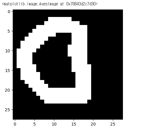
# 전처리
# 이미지 컬러이미지 > 흑백이미지로 변경
img = img.convert('L')

# 이미지데이터를 2배열로 변환
img = np.array(img)
img.shape
# 완본 이미자에 했던 전처리를 그대로 해주어야한다
# 2차원 -> 1 차원 (flatten)
testimg = img.reshape(1,28,28,1)
testimg.astype('float32')/255
testimg.shape
# 우리의best_model 불러와사 확인하기
from tensorflow.keras.models import load_model
best_model = load_model('/content/drive/MyDrive/Colab Notebooks/Deep Learning/data/best_model/bm_34_0.97.hdf5')best_model.evaluate(x_test,y_test)
# 우리의 손글씨 넣어서 예측하기
best_model.predict(testimg)
# 10개의 확률값 출력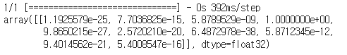
# 하나의 클래스를 출력하고 싶다면?
best_model.predict(testimg).argmax()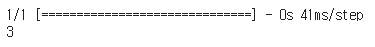
img = pimg.open('/content/drive/MyDrive/Colab Notebooks/Deep Learning/data/손글씨/5.png')
plt.imshow(img,cmap = 'gray')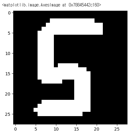
best_model.predict(testimg)best_model.predict(testimg).argmax()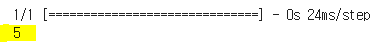
정리
- test데이터 대해서는 높은 성능을 보였으나
- 우리가 작성한 송글씨에서는 낮은 점확도를 보이더라
- 제공된 데이터는 데이터의 크기와 모양이 일정하게 정제되어았음
- 하지만 우리의 데이터는 모양와 위치가 학습데이터와 일치하지 않기 때문에 결과가 별로
- Dense 층은 1차원데이터만 학습이 가능하더라
- 이미지는 2차원 데이터 (우리가 억지로 1차원으로 만들어서 학습)

열심히 공부합시다! The best is yet to come! 💜