👨‍🏫학습목표

오늘은 DPG와 DDPG의 개념에 대해 배워볼 예정이다.

👨‍🎓강의영상: https://www.youtube.com/watch?v=Ukloo2xtayQ

1️⃣ Deep Deterministic Policy Gradient

🔷 기존의 모델

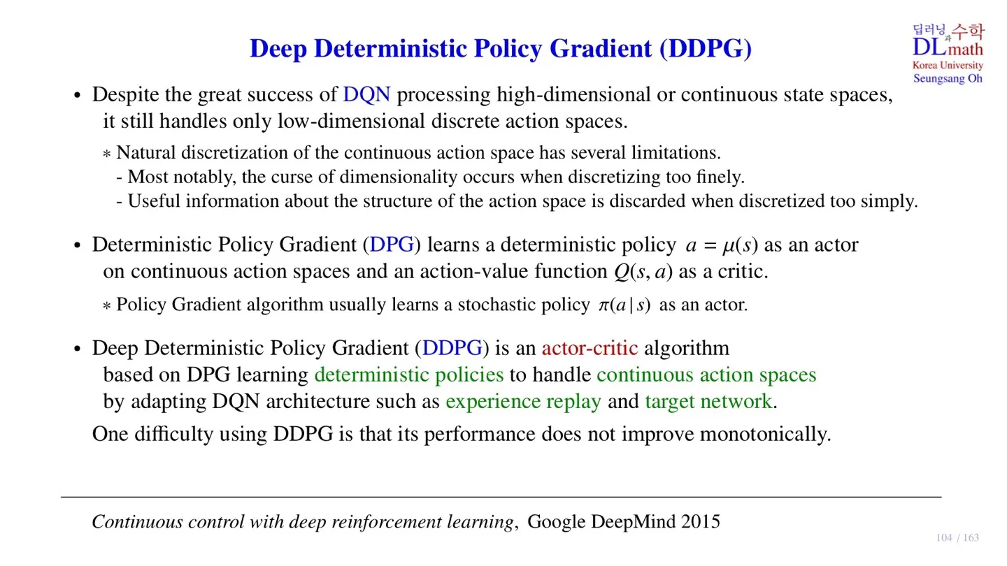
🔻 DQN

• 크고 continuous한 state space를 입력으로 처리할 수 있다.
• 하지만 출력으로는 작고 discrete한 action space만 처리할 수 있어서 로보틱스에 적용하기 힘들었다.

🔻 A3C

• Policy를 직접 approximation하기 때문에 Continuous action space를 처리할 수 있다.

지금까지 다루었던 Stochastic policy $\pi(a|s)$ 는 random한 성질이 반영되었다.
오늘은 다른 방법으로 continuous action space를 처리할 수 있는 모델을 다뤄보려 한다.

🔷 Deterministic Policy Gradient (DPG)

• Deterministic policy $a = \mu(s)$ 를 배운다.
• Deterministic policy는 입력 state가 주어지면 action이 결정된다.
• Actor : deterministic policy $a = \mu(s)$
• Critic : action-value function $Q(s,a)$

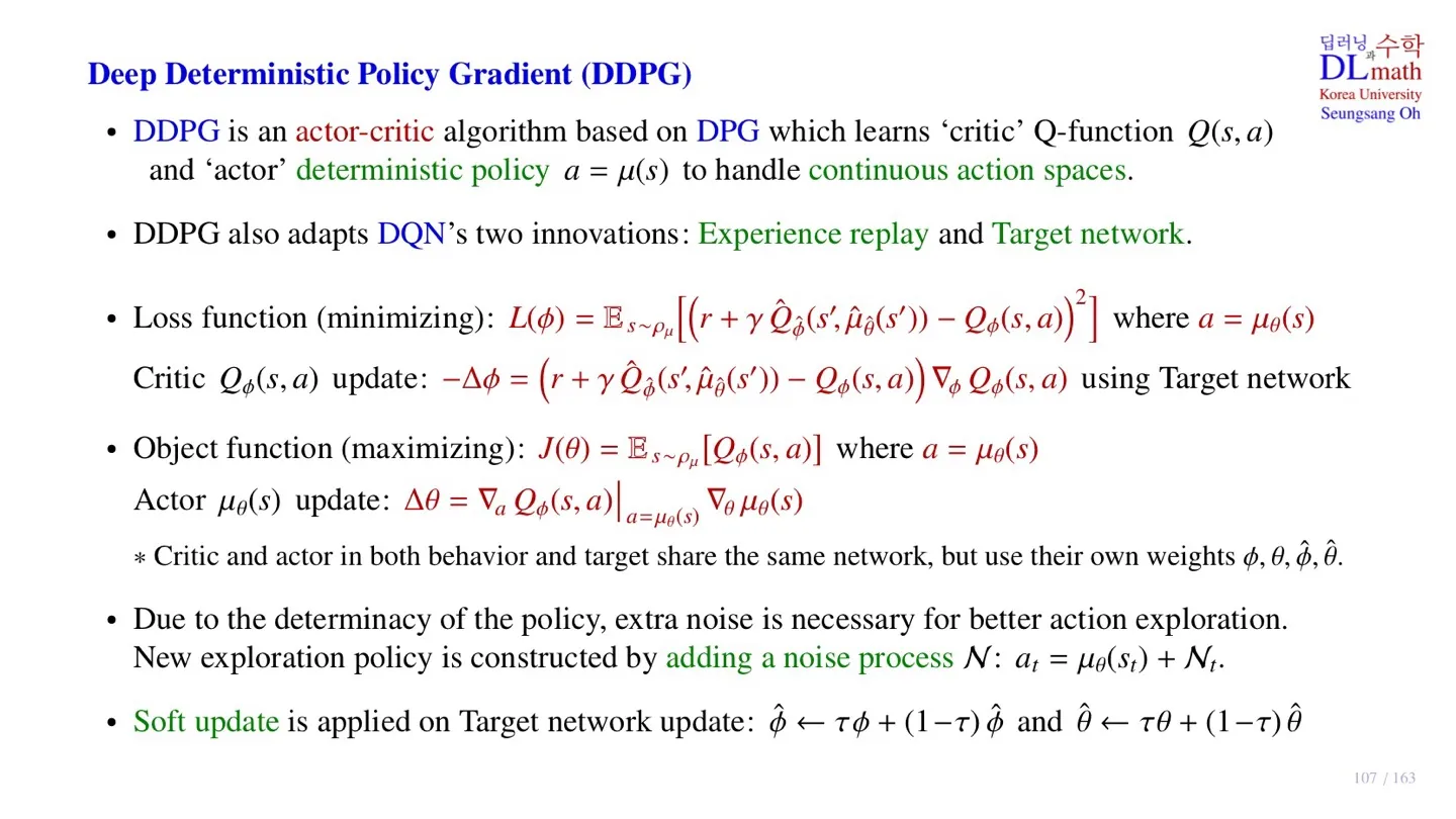
🔷 Deep Deterministic Policy Gradient (DDPG)

• DPG를 기반으로 한 Actor-critic algorithm
• Deterministic policy를 학습한다.
• $Q(s,a)$를 구하기 위해 DQN을 사용한다.
• DQN을 사용하기 때문에 DQN의 핵심 구조인 experience ereplay와 target network 역시 사용한다.
• 다만 학습이 진행됨에 따라 반드시 Object function이 개선되지는 않는다는 한계가 존재한다.

---

2️⃣ Deterministic Policy Gradient

🔷 DPG

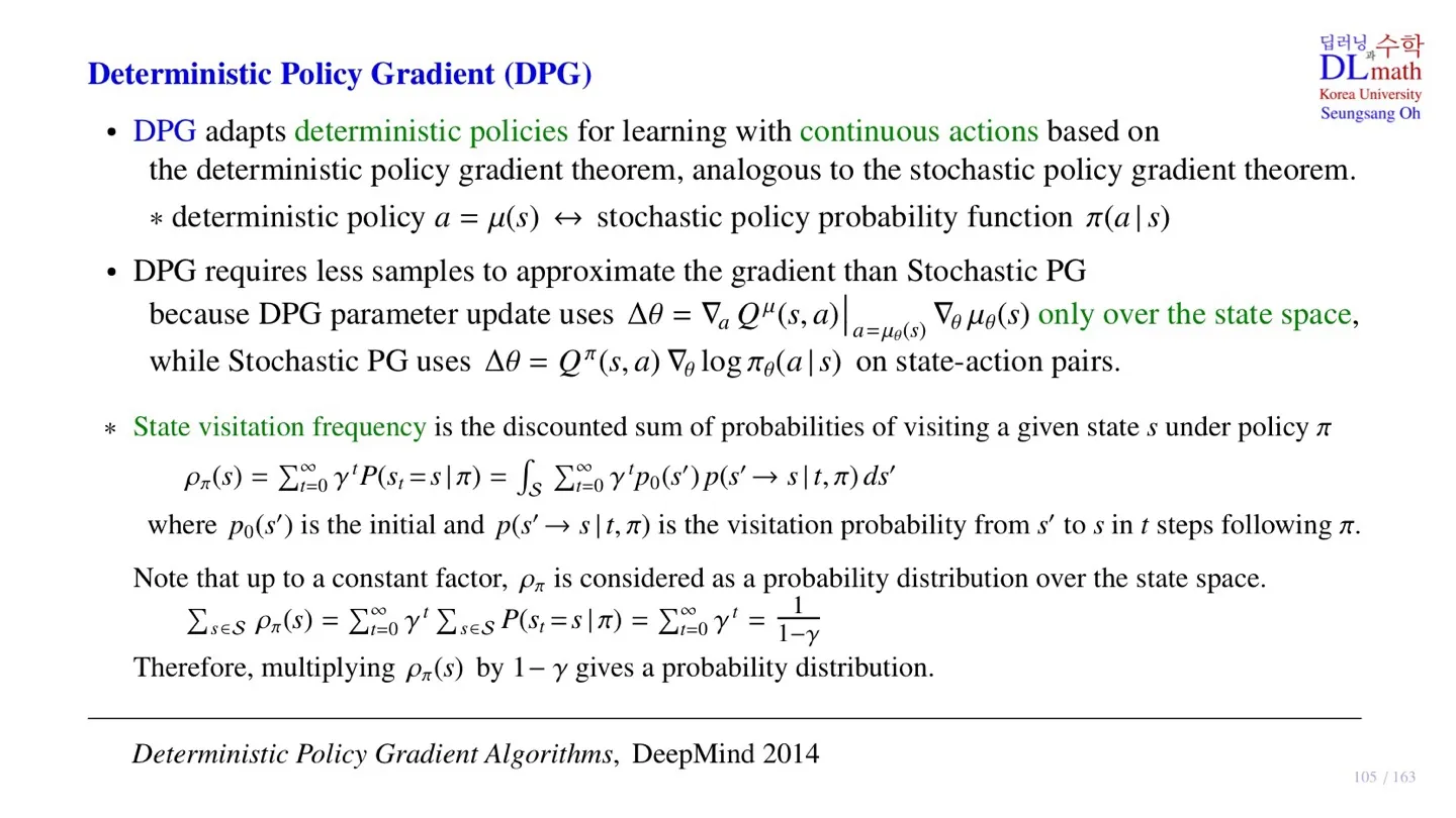
• Continous action space를 처리하기 위해 deterministic policy를 사용한다.
• Deterministic policy $a = \mu(s)$

🔻 DPG의 gradient

$\Delta \theta = \nabla_a Q^\mu(s, a)|_{a=\mu_\theta(s)} \nabla_\theta \mu_\theta(s)$

• State에 대해 action이 deterministic하게 결정되기 때문에 state만 고려하면 된다.
• 즉 훨씬 더 적은 데이터로 학습이 가능하다.

🔻 State visitation frequency

• 주어진 Policy에서 특정한 state를 얼마나 자주 방문하는지 알려주는 값이다.

$\rho_\pi(s) = \sum_{t=0}^{\infty} \gamma^t P(S_t = s | \pi) = \int_\mathcal{S} \sum_{t=0}^{\infty} \gamma^t p_0(s') p(s' \to s | t, \pi) ds'$

• $\rho_\pi(s):$ 주어진 policy에서 해당 state의 state visitation frequency
• 주어진 policy에서 특정 state가 발생할 확률을 discount factor로 가중합한 값이다.
• 모든 시점 $t$에서 해당 특정 state가 발생할 확률을 더한다.
• $p_0(s'):$ $s'$ 에서 시작할 확률
• $p(s' \to s | t, \pi):$ 시점 $t$에서 $s$에 도달할 확률
• $\int_\mathcal{S} ds':$ 모든 state가 시작 state $s'$가 될 수 있고 state space가 continuous하기 때문에 적분한다.

$\sum_{s \in \mathcal{S}} \rho_\pi(s) = \sum_{t=0}^\infty \gamma^t \sum_{s \in \mathcal{S}} P(S_t = s | \pi) = \sum_{t=0}^\infty \gamma^t = \frac{1}{1-\gamma}$

• $\sum_{t=0}^\infty ,\sum_{s \in \mathcal{S}}$의 순서를 바꾸어도 식은 성립한다.
• $\sum_{s \in \mathcal{S}} P(S_t = s | \pi)=1$ 이므로 두번째 등호가 성립한다.
• $\sum_{s \in \mathcal{S}} \rho_\pi(s) = \frac{1}{1-\gamma}$ 이므로 $\rho_\pi(s)$에 $1-\gamma$를 곱하면 확률로 만들 수 있다.

---

3️⃣ Stochastic VS Deterministic

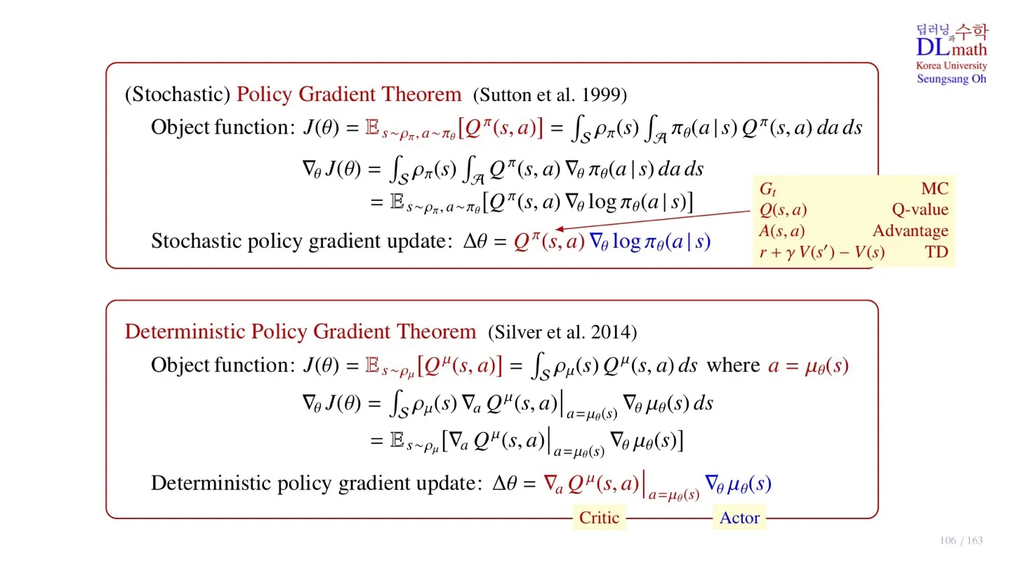
🔷 Stochactic Policy Gradient Theorem

🔻 Object function

$J(\theta) = \mathbb{E}_{s \sim \rho_\pi, a \sim \pi_\theta}[Q^\pi(s, a)] = \int_\mathcal{S} \rho_\pi(s) \int_\mathcal{A} \pi_\theta(a|s) Q^\pi(s, a) da ds$

• Q-function의 기대값을 object function으로 사용한다.
• $s \sim \rho_\pi:$ State는 state visitation frequency를 따른다.
• $a \sim \pi_\theta:$ Action은 policy를 따른다.
• $\mathbb{E}_{s \sim \rho_\pi, a \sim \pi_\theta}[...]:$ State와 Action에 대해 둘다 기대값을 적용해야 하기 때문에 $\int_\mathcal{S} \int_\mathcal{A} ... da ds$ 를 적용한다.

🔻 Gradient

$\nabla_\theta J(\theta) = \int_\mathcal{S} \rho_\pi(s) \int_\mathcal{A} Q^\pi(s, a) \nabla_\theta \pi_\theta(a|s) da ds$

$= \mathbb{E}_{s \sim \rho_\pi, a \sim \pi_\theta}[Q^\pi(s, a) \nabla_\theta \log \pi_\theta(a | s)]$

🔻 Stochastic policy gradient update

$\Delta \theta = Q^\pi(s, a) \nabla_\theta \log \pi_\theta(a | s)$

• Critic : $Q^\pi(s, a)$
• Actor : $\nabla_\theta \log \pi_\theta(a | s)$

🔷 Deterministic Policy Gradient Theorem

🔻 Object function

$J(\theta) = \mathbb{E}_{s \sim \rho_\mu}[Q^\mu(s, a)] = \int_\mathcal{S} \rho_\mu(s) Q^\mu(s, a) ds \quad \text{where } a = \mu_\theta(s)$

• Q-function의 기대값을 object function으로 사용한다.
• $s \sim \rho_\pi:$ State는 state visitation frequency를 따른다.
• $a = \mu_\theta(s):$ Action은 state에 따라 deteministic하게 결정된다.
• $\mathbb{E}_{s \sim \rho_\pi}[...]:$ State에 대해 기대값을 적용해야 하기 때문에 $\int_\mathcal{S} ... ds$ 를 적용한다.

🔻 Gradient

$\nabla_\theta J(\theta) = \int_\mathcal{S} \rho_\mu(s) \nabla_a Q^\mu(s, a)|_{a=\mu_\theta(s)} \nabla_\theta \mu_\theta(s) ds$

$= \mathbb{E}_{s \sim \rho_\mu}[\nabla_a Q^\mu(s, a)|_{a=\mu_\theta(s)} \nabla_\theta \mu_\theta(s)]$

🔻 Deterministic policy gradient update

$\Delta \theta = \nabla_a Q^\mu(s, a)|_{a=\mu_\theta(s)} \nabla_\theta \mu_\theta(s)$

• Critic : $\nabla_a Q^\mu(s, a)|_{a=\mu_\theta(s)}$
• Actor : $\nabla_\theta \mu_\theta(s)$

---

4️⃣ Deep Deterministic Policy Gradient

🔷 DDPG

• DPG를 기반으로 한 actor-critic algorithm이다.
• Critic으로는 Q-function $Q(s,a)$를 학습한다.
• Actor로는 deterministic policy $a = \mu(s)$를 학습한다.
• Critic Network로는 DQN을 사용하며, 따라서 DQN의 experience replay와 Target Network 구조 역시 사용한다.

🔻 Critic Network의 Loss function

$L(\phi) = \mathbb{E}_{s \sim \rho_\mu}\left[ \left[r + \gamma \hat{Q}_{\hat{\phi}}(s', \hat{\mu}_{\hat{\theta}}(s')) - Q_\phi(s, a)\right]^2 \right] \text{ where } a = \mu_\theta(s)$

• DQN과 동일한 Loss을 적용한다.
• Temporal Difference error를 사용한다.
• Target Network와 behavior Network가 구분되어 있는 Off-policy이다.
• 단, Action은 actor Network에서 deterministic하게 결정된다.

🔻 Critic Network 업데이트

$-\Delta\phi = (r + \gamma \hat{Q}_{\hat{\phi}}(s', \hat{\mu}_{\hat{\theta}}(s')) - Q_\phi(s, a)) \nabla_\phi Q_\phi(s, a)$

• Gradient descent 방식으로 업데이트한다.

🔻 Actor Network의 Object function

$J(\theta) = \mathbb{E}_{s \sim \rho_\mu}[Q_\phi(s, a)] \text{ where } a = \mu_\theta(s)$

🔻 Actor Network 업데이트

$\Delta \theta = \nabla_a Q_\phi(s, a)|_{a=\mu_\theta(s)} \nabla_\theta \mu_\theta(s)$

• Gradient ascent 방식으로 업데이트한다.

🔷 학습 파라미터

• $\phi, \theta, \hat{\phi}, \hat{\theta}$ 총 4개를 사용한다.
• Action이 deterministic하기 때문에 exploration이 부족하다는 한계가 존재한다.
• 이를 위해 출력된 action에 noise를 더하는 방법을 사용한다.

$\mathcal{N}: a_t = \mu_\theta(s_t) + \mathcal{N}_t$

• 각 step마다 다른 noise를 부여하기 위해 Noise squence를 만든다.
• 그리고 해당 step $t$에 맞는 noise $\mathcal{N}_t$ 를 더한다.

🔻 Target Network의 soft update

$\hat{\phi} \leftarrow \tau\phi + (1-\tau)\hat{\phi} \text{ and } \hat{\theta} \leftarrow \tau\theta + (1-\tau)\hat{\theta}$

• 기존의 DQN은 일정 step 후 target Network를 behavior Network로 업데이트한다.
• 일정 step마다 parameter를 조금씩 업데이트한다.

---

5️⃣ DDPG의 pseudo code

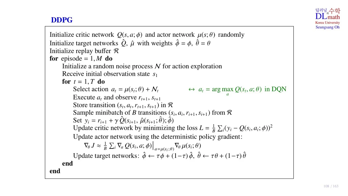
🔷 초기 설정

🔻 파라미터 초기화

• Critic Network $Q(s,a;\phi)$와 Actor Network $\mu(s;\theta)$를 초기화한다.
• Target Network $\hat{\phi}=\phi, \hat{\theta}=\theta$로 초기화한다.
• Replay Buffer $\mathcal{R}$ 을 정의한다.

🔷 업데이트 진행

🔻 Noise sequence, 시작 state 초기화

• Initial state $s_1$ 설정
• Noise sequence $\mathcal{N}$ 초기화

🔻 Sample data 수집

• Deterministic policy $\mu(s_t;\theta)$을 통해 action 선정
• $a_t = \mu(s_t;\theta) + \mathcal{N}_t$ noise를 추가하여 action 변형
• Action $a_t$를 통해 immediate reward $r_{t+1}$과 next state $s_{t+1}$ 수집
• $(s_t, a_t, r_{t+1}, s_{t+1})$을 replay buffer $\mathcal{R}$에 저장한다.

🔻 파라미터 업데이트

• Replay buffer $\mathcal{R}$ 에서 minibatch $\mathcal{B}$ 만큼 sample data를 추출한다.
• Sample data를 통해 target $y_i = r_{i+1} + \gamma \hat{Q}(s_{i+1}, \hat{\mu}(s_{i+1}; \hat{\theta}); \hat{\phi})$를 구한다.

$L = \frac{1}{B} \sum_i (y_i - Q(s_i, a_i; \phi))^2$

• Target을 통해 critic Network를 업데이트한다.

$\nabla_\theta J \approx \frac{1}{B} \sum_i \left.\nabla_a Q(s_i, a; \phi)\right|_{a=\mu(s_i; \theta)} \nabla_\theta \mu(s_i; \theta)$

• Deterministic policy gradient를 사용하여 Actor Network도 업데이트한다.

$\hat{\phi} \leftarrow \tau\phi + (1-\tau)\hat{\phi} \text{ and } \hat{\theta} \leftarrow \tau\theta + (1-\tau)\hat{\theta}$

• 일정 step이 지난 후 target Network를 soft update를 진행한다.

---

6️⃣ 정리

🔷 26강에서 배운 내용은 아래와 같다.

1. DPG는 deterministic policy를 사용한다.
2. DDPG는 DPG를 기반으로 한 actor-acritic algorithm이다.
3. DDPG는 Replay Buffer를 사용한다.
4. DDPG는 target Network와 behavior Network가 분리되어 있는 off-policy이다.
5. DDPG는 target Network를 업데이트할 때, soft updata를 진행한다.