👨‍🏫학습목표

오늘은 TRPO의 개념과 TRPO의 object function에 대해 배워볼 예정이다.

👨‍🎓강의영상: https://www.youtube.com/watch?v=c15b9AjHxBA

TRPO 논문: https://arxiv.org/pdf/1502.05477

Conservative policy iteration update 논문: https://arxiv.org/pdf/1906.09784

1️⃣ Trust Region Policy Optimization

📕 지난시간에 배운 내용 DDPG

• Continuous action space를 다루기 위해서 deterministic policy $\mu(s)$를 사용한다.
• 하지만 monotonically improve가 되지 않는다.

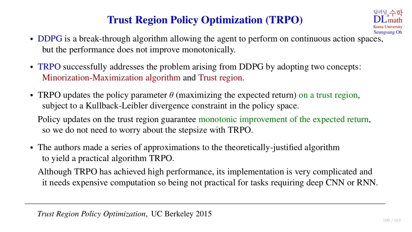
🔷 TRPO

• DDPG의 한계를 극복하기 위해 TRPO는 2가지 개념을 채택한다.
• 첫 번째는 Minorization-Maximization algorithm이다.
• 두 번째는 Trust region이다.
• TRPO는 policy parameter를 trust region에서 업데이트한다.
• Trust region은 KL-divergence를 제약조건으로 만든다.
• Trust region에서의 parameter 업데이트는 expected return의 monotonic improvement를 보장한다.
• Monotonic improvement가 보장되어 step size에 대해 고민할 필요가 없다.

🔻 TRPO의 특징

• TRPO는 등장 논문에서 이론적으로 정립되었지만, 실제로 적용하는 것에는 어려움이 있었다.
• 따라서 논문의 저자는 여러 approximation을 통해 TRPO를 구현하였다.
• TRPO는 좋은 성능을 발휘하지만, Network의 scale이 커지면 구현하는 데 어려움이 있다.
• 이미지 데이터는 CNN을, sequential data는 RNN을 사용하지만 Network의 크기가 너무 커지면 안된다.

---

2️⃣ Trust Region에 대한 Intuition

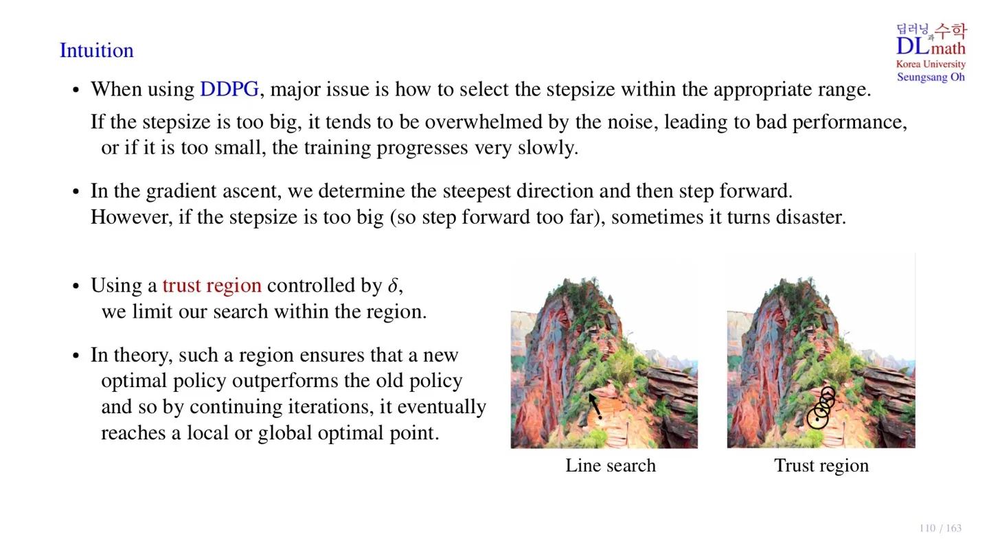
🔷 Trust Region 사용 이유

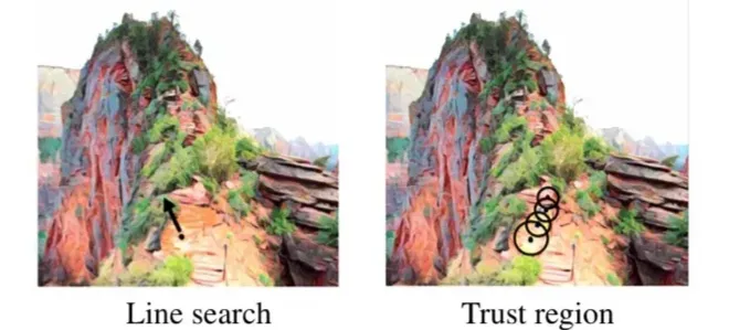
• 목표는 산 정상에 가는 것이다. 이는 Object function을 최대화하는 것과 같다.
• 왼쪽 그림에서 언덕을 올라가기 위해 gradient를 계산하면 가장 경사가 높은 방향으로 이동할 것이다.
• 하지만 너무 많이 이동하게 되면 낭떨어지로 떨어질 수도 있다.
• 오른쪽 그림처럼 이동을 해도 안전하고 올라간다는 보장이 있는 영역을 만든다면 이동 보폭과 관계없이 편하게 이동할 수 있다.

🔻 TRPO의 한계 다시 정리

• Object function을 maximize하는 방향을 알지만 step size를 알 수 없다.
• Step size가 너무 클 경우 성능이 떨어지는 문제가 존재한다.
• Step size를 작게 하면 안전할 수 있지만, 학습 속도가 느려진다.

🔷 TRPO의 Trust Region

• $\delta$를 이용하여 trust region의 크기를 조절한다.
• Trust region 안에서 new optimal policy를 찾게 되면 이전 policy보다 성능이 더 좋다.
• Trust region에서 optimal policy를 찾는 과정을 반복하면 global or local policy에 도달할 수 있다.
• TRPO에서 가장 중요한 것을 trust region을 찾는 것이다.

---

3️⃣ TRPO의 Object function 1

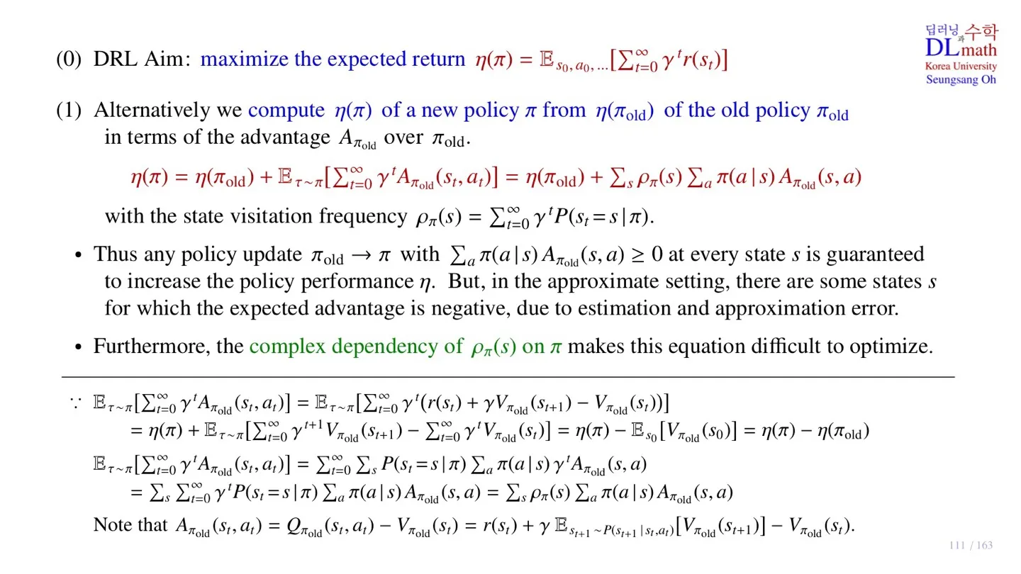
🔷 Object function

$\eta(\pi) = \mathbb{E}_{s_0, a_0, \dots}\left[\sum_{t=0}^{\infty} \gamma^t r(s_t)\right]$

• 현재 주어진 policy $\pi$를 통해 episode 데이터를 수집한다.
• 수집한 데이터를 통해 구한 expected return을 object function으로 한다.
• Object function을 maximize하는 방향으로 policy를 업데이트한다.

🔷 Object function 구하기

• 업데이트된 policy의 $\eta(\pi)$를 구하기 위해서 기존의 policy $\pi_{old}$의 $\eta(\pi_{old})$ 값을 활용한다.

$\eta(\pi) = \eta(\pi_\text{old}) + \mathbb{E}_{\tau \sim \pi}\left[\sum_{t=0}^{\infty} \gamma^t A_{\pi_\text{old}}(s_t, a_t)\right]$

$\eta(\pi_\text{old}) + \mathbb{E}_{\tau \sim \pi}\left[\sum_{t=0}^{\infty} \gamma^t A_{\pi_\text{old}}(s_t, a_t)\right] = \eta(\pi_\text{old}) + \sum_{s} \rho_\pi(s) \sum_a \pi(a|s) A_{\pi_\text{old}}(s,a)$

• 각 식에서 우변의 2번째 항에 대해 집중해서 살펴볼 필요가 있다.

🔻 첫 번째 등호 증명하기

$\mathbb{E}_{\tau \sim \pi}[\sum_{t=0}^{\infty} \gamma^t A_{\pi_\text{old}}(s_t, a_t)] = \mathbb{E}_{\tau \sim \pi}[\sum_{t=0}^{\infty} \gamma^t (r(s_t) + \gamma V_{\pi_\text{old}}(s_{t+1}) - V_{\pi_\text{old}}(s_t))]$

• 좌변의 Advantage function $A_{\pi_\text{old}}(s_t, a_t)$는 $r(s_t) + \gamma V_{\pi_\text{old}}(s_{t+1}) - V_{\pi_\text{old}}(s_t)$로 바꿀 수 있다.

$\mathbb{E}_{\tau \sim \pi}[\sum_{t=0}^{\infty} \gamma^t (r(s_t) + \gamma V_{\pi_\text{old}}(s_{t+1}) - V_{\pi_\text{old}}(s_t))]$

$\mathbb{E}_{\tau \sim \pi}[\sum_{t=0}^{\infty} \gamma^t (r(s_t)] = \eta(\pi)$

• $\mathbb{E}_{\tau \sim \pi}$ 속 첫 번째 항은 Object function으로 바꿀 수 있다.

$\mathbb{E}_{\tau \sim \pi}[\sum_{t=0}^{\infty} \gamma^t (r(s_t) + \gamma V_{\pi_\text{old}}(s_{t+1}) - V_{\pi_\text{old}}(s_t))] = \eta(\pi) + \mathbb{E}_{\tau \sim \pi}[\sum_{t=0}^{\infty} \gamma^{t+1} V_{\pi_\text{old}}(s_{t+1}) - \sum_{t=0}^{\infty} \gamma^t V_{\pi_\text{old}}(s_t)]$

• 따라서 위 식으로 변환이 가능하다.
• 이때 $\sum_{t=0}^{\infty}\gamma^{t+1} V_{\pi_\text{old}}(s_{t+1}) - \sum_{t=0}^{\infty} \gamma^t V_{\pi_\text{old}}(s_t)$값은 $t$가 증가함에 따라 서로 상쇄되는 것을 확인할 수 있다.

$\eta(\pi) + \mathbb{E}_{\tau \sim \pi}[\sum_{t=0}^{\infty} \gamma^{t+1} V_{\pi_\text{old}}(s_{t+1}) - \sum_{t=0}^{\infty} \gamma^t V_{\pi_\text{old}}(s_t)] = \eta(\pi) - \mathbb{E}_{s_0}[V_{\pi_\text{old}}(s_0)]$

$\eta(\pi) - \mathbb{E}_{s_0}[V_{\pi_\text{old}}(s_0)] = \eta(\pi) - \eta(\pi_\text{old})$

• $\mathbb{E}_{s_0}$ 는 모든 state를 시작 지점으로 얻을 수 있는 return의 expectation을 의미하는데, 이는 정의에 따라 $\eta(\pi_{old})$로 바꿀 수 있다.

$\mathbb{E}_{\tau \sim \pi}\left[\sum_{t=0}^{\infty} \gamma^t A_{\pi_\text{old}}(s_t, a_t)\right] = \eta(\pi)- \eta(\pi_\text{old})$

• 따라서 위 식이 성립하므로 첫 번째 등호가 성립한다.

🔻 두 번째 등호 증명하기

$\rho_\pi(s) = \sum_{t=0}^{\infty} \gamma^t P(s_t = s | \pi)$

• $\rho_\pi(s)$는 state visitation frequency를 의미한다.

$\eta(\pi_\text{old}) + \mathbb{E}_{\tau \sim \pi}\left[\sum_{t=0}^{\infty} \gamma^t A_{\pi_\text{old}}(s_t, a_t)\right] = \eta(\pi_\text{old}) + \sum_{s} \rho_\pi(s) \sum_a \pi(a|s) A_{\pi_\text{old}}(s,a)$

• 여기서 좌변의 2번째 항에 대해 살펴보자.

$\mathbb{E}_{\tau \sim \pi}[\sum_{t=0}^{\infty} \gamma^t A_{\pi_\text{old}}(s_t, a_t)] = \sum_{t=0}^{\infty} \sum_s P(s_t = s | \pi) \sum_a \pi(a|s) \gamma^t A_{\pi_\text{old}}(s, a)$

• $\mathbb{E}_{\tau \sim \pi} \ ,\sum_{t=0}^{\infty}$ 의 순서를 바꿀 수 있다.
• $\mathbb{E}_{\tau \sim \pi}$ 은 $\sum_s P(s_t = s | \pi) \sum_a \pi(a|s)$ 로 풀어서 적을 수 있다.

$= \sum_s \sum_{t=0}^{\infty} \gamma^t P(S_t=s|\pi) \sum_a \pi(a|s) A_{\pi_\text{old}}(s,a) = \sum_s \rho_\pi(s) \sum_a \pi(a|s) A_{\pi_\text{old}}(s,a)$

• $\sum_{t=0}^{\infty}$ 에 대한 순서를 바꿔주면 최종적으로 $\rho_\pi(s)$를 구할 수 있다.

$\mathbb{E}_{\tau \sim \pi}[\sum_{t=0}^{\infty} \gamma^t A_{\pi_\text{old}}(s_t, a_t)] = \sum_s \rho_\pi(s) \sum_a \pi(a|s) A_{\pi_\text{old}}(s, a)$

• 따라서 위 식이 성립하므로 두 번째 등호가 만족한다

🔻 Object function 이해하기

$\eta(\pi) = \eta(\pi_\text{old}) + \sum_{s} \rho_\pi(s) \sum_a \pi(a|s) A_{\pi_\text{old}}(s,a)$

• New policy의 $\eta(\pi)$를 구하기 위해서 $\eta(\pi_{old})$에 2번째 항을 더한다.

🔷 Objection function의 optimize

$\eta(\pi) = \eta(\pi_\text{old}) + \sum_{s} \rho_\pi(s) \sum_a \pi(a|s) A_{\pi_\text{old}}(s,a)$

• 위 식을 통해 object function을 maximize하기 위해서는 $\eta(\pi) \geq \eta(\pi_\text{old})$가 보장되어야 한다.
• $\rho_\pi(s) \geq 0:$ $\rho_\pi(s)$은 확률값이기 때문에 0보다 크다.
• 따라서 $\sum_a \pi(a|s) A_{\pi_\text{old}}(s,a) \geq 0$ 를 만족하면 object function을 업데이트 할수록 성능이 개선됨을 증명할 수 있다.

🔻 한계

• 하지만 간혹 $\sum_a \pi(a|s) A_{\pi_\text{old}}(s,a) \leq 0$ 인 경우가 존재하여 아직까지 성능이 계속 향상됨을 증명할 수 없다.
• 또한 $\rho_\pi(s)$를 구하기 위해서 new policy $\pi$의 sample state를 수집해야 하는데, 아직까지 new policy를 구하는 과정이기 때문에 실제로 sample state를 수집할 수 없다.
• 따라서 위 식에 있는 new policy를 old policy $\pi_{old}$ 로 바꿔야 한다.
• 이 과정이 첫 번째 approximation이다.

---

4️⃣ TRPO의 Object function 2

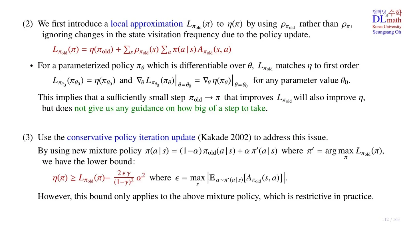
🔷 Object function approximation

$L_{\pi_\text{old}}(\pi) = \eta(\pi_\text{old}) + \sum_s \rho_{\pi_\text{old}}(s) \sum_a \pi(a|s) A_{\pi_\text{old}}(s, a)$

• $L_{\pi_\text{old}}(\pi):$ 근사한 Object function
• 기존 식의 $\rho_{\pi}(s)$를 $\rho_{\pi_\text{old}}(s)$으로 변환한 것을 확인할 수 있다.

🔻 그래프로 확인

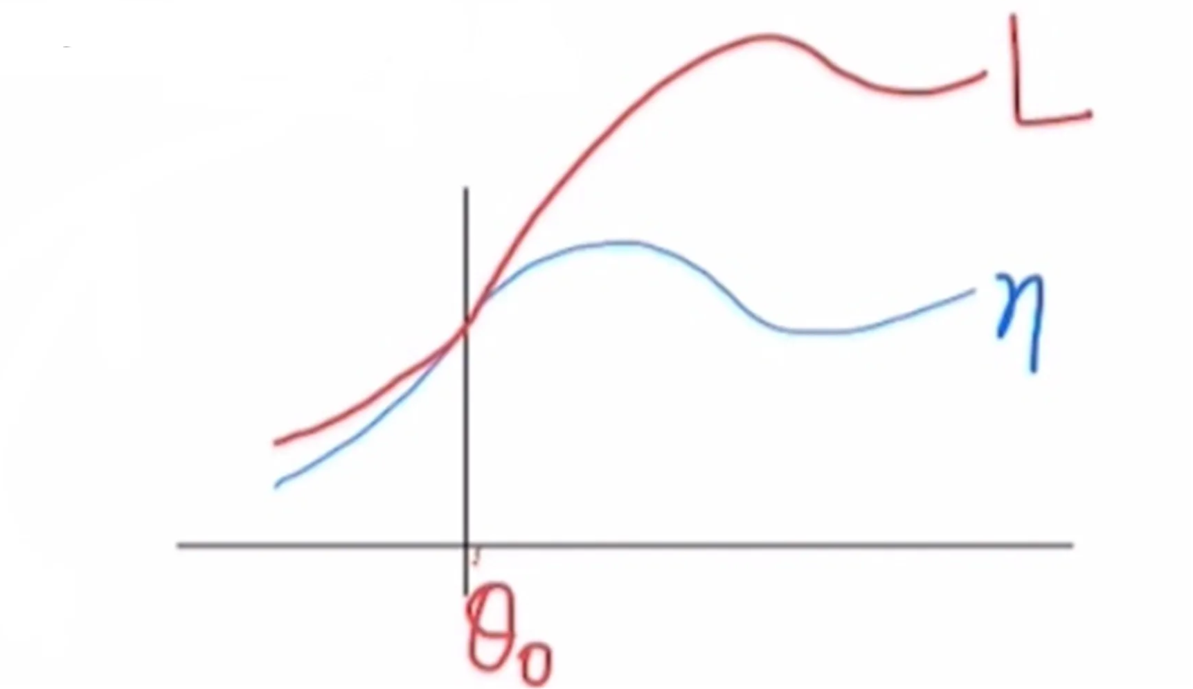
• 근사를 할 경우 그림처럼 표현할 수 있다.
• Old policy $\pi_{old}$의 파라미터를 $\theta_0$라 할 때, 원래 식과 근사한 식이 $\theta_0$에서 유사한 것을 확인할 수 있다.
• Old policy $\pi_{old}$와 new policy $\pi$가 local한 영역에서 유사하게 움직인다.

🔻 수식으로 확인

$L_{\pi_{\theta_0}}(\pi_{\theta_0}) = \eta(\pi_{\theta_0}) \text{ for any parameter value } \theta_0.$

🔸 위 식에 성립하는 이유

$L_{\pi_\text{old}}(\pi) = \eta(\pi_\text{old}) + \sum_s \rho_{\pi_\text{old}}(s) \sum_a \pi(a|s) A_{\pi_\text{old}}(s, a)$

• 위 식의 좌변에서 $\pi$자리에 $\pi_{\theta_0}$를 넣게 되면 우변 2번째 항의 $\pi(a|s)$가 $\pi_\text{old}(a|s)$가 된다.
• 그 결과 $\sum_a \pi_\text{old}(a|s) A_{\pi_\text{old}}(s, a)$가 만들어지는데 $\sum_a \pi_\text{old}(a|s) A_{\pi_\text{old}}(s, a)=0$이 성립한다.
• 따라서 위 식이 유도된다.

$\nabla_\theta L_{\pi_{\theta_0}}(\pi_{\theta_0})|_{\theta=\theta_0} = \nabla_\theta \eta(\pi_\theta)|_{\theta=\theta_0} \text{ for any parameter value } \theta_0.$

• Gradient가 유사하기 때문에 근사식이 improve되는 방향에서 기존의 식 역시 improve될 수 있음을 알 수 있다.
• 다만 근사한 영역의 크기를 알 수는 없기에 step size에 대한 정보는 알 수 없다.
• 이를 해결하기 위해 여러 단계를 다룬다.

🔷 Conservative policy iteration update

$\pi(a|s) = (1-\alpha)\pi_\text{old}(a|s) + \alpha\pi'(a|s) \text{ where } \pi' = \arg\max_\pi L_{\pi_\text{old}}(\pi)$

• Conservative policy iteration update는 근사식 $L_{\pi_\text{old}}(\pi)$을 최적화시킨 후 그 값을 Old policy $\pi_{old}$에 일부만 반영하는 방법이다.

$\eta(\pi) \geq L_{\pi_\text{old}}(\pi) - \frac{2\epsilon\gamma}{(1-\gamma)^2}\alpha^2 \text{ where } \epsilon = \max_s |\mathbb{E}_{a \sim \pi'(a|s)}[A_{\pi_\text{old}}(s,a)]|$

• Conservative policy iteration update을 사용하면 업데이트된 policy가 lower bound를 가진다.
• $\alpha$값이 커질수록 lower bound가 낮아진다.
• Discount factor $\gamma$가 1에 가까워질수록 lower bound가 낮아진다.
• 하지만 $\epsilon$ 값을 구하는 것은 쉽지 않다.
• 또한 mixture policy라는 개념 역시 아직까지 practical하게 적용하기는 쉽지 않다.

---

5️⃣ 정리

🔷 27강에서 배운 내용은 아래와 같다.

1. TRPO는 DDPG가 monotinic하게 improve되지 않는다는 한계를 극복하기 위해 등장하였다.
2. TRPO는 Trust region과 Minorization-Maximization algorithm이 사용된 모델이다.
3. TRPO는 expected return을 object function으로 사용한다.
4. TRPO의 object function을 구하기 위해서는 여러 approximation을 거쳐야 한다.
5. Conservative policy iteration update는 lower bound를 보장하지만 구현하기가 어렵다.