🧑‍🎓 나의 AI 기록

2018, 2019년도 학부수업에서 딥러닝을 처음 접했다. 파이썬을 배운지 얼마되지 않은 학부생에게 layer, optimization, validation, 등 개념들은 혼란스러웠다. 이후 학부 졸업논문으로 '딥러닝 기반 미세먼지 (PM10) 6시간-시계열 예측 모델 비교' 라는 주제를 다루었다. 그리고 석사 1기 동안 《PyTorch를 활용한 강화학습/심층강화학습 실전 입문》를 교재로 강화학습도 접해보았다.

🩻이번에는 이미지 !

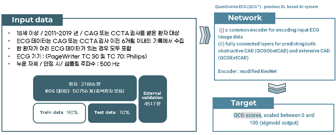
최근 심전도(EKG, ECG)-AI 논문들을 접하였고 연속적인 파동 데이터를 학습하는 줄 알았지만 12-lead ECG 이미지를 통으로 학습해도 유의미한 결과가 나오는 것을 확인했다.

Jiesuck Park, et al. Artificial intelligence–enhanced electrocardiography analysis as a promising tool for predicting obstructive coronary artery disease in patients with stable angina. European Heart Journal - Digital Health (2024) 00, 1–10 .

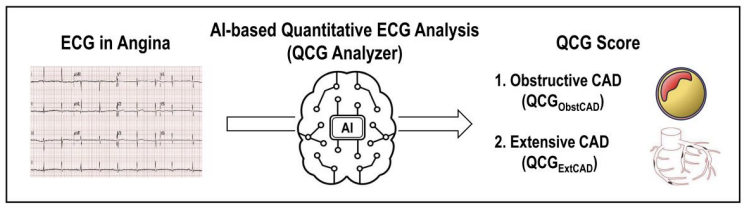
위 논문에서는 modified ResNet 을 선택하여 0 ~ 100 사이의 QCG score 를 도출해는 방법을 연구하였다. 여기서 QCG score 는 급성관상동맥증후군, 심근경색 등 심혈관질환을 예측하기 위해 만들어진 지표이다.

논문을 읽으면서 p-value, $\chi^2$-test, AUC 등 평가지표를 포함하여 모르는 내용들이 많았지만 우선 모델인 ResNet 부터 공부해보려한다.

🤖 ResNet

Kaiming He, Xiangyu Zhang, Shaoqing Ren, Jian Sun. Deep Residual Learning for Image Recognition. arXiv:1512.03385

Motivation

마이크로소프트사에서 개발된 ResNet 은 이미지 분류 모델로 당시 CNN의 점점 깊어지는 network가 계속해서 좋은 성능을 보이자 다음과 같은 의문점에서 시작되었다.

"Is learning better networks as easy as stacking more layers?"

이 질문은 기울기 소실/폭증 문제(problem of vanishing/exploding gradients)를 어떻게 해결하는지에 달려있었고 Stochastic Gradient Descent(SGD)로 보안될 수 있었다.
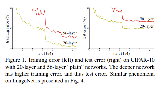
다음으로 layer 를 더 깊게 설정했을 때, 네트워크가 수렴하다가 정확도가 저하되는 순간의 문제를 포착하였고 나아가 더 깊은 모델일수록 학습 오차가 커지는 것을 알 수 있었다.

더 깊은 모델의 구상으로 shallower architecture 와 그 뒤로 identity mapping 을 붙이는 것으로 선택하였다. shallower architecture 의 출력값을 그대로 복사하는 identity mapping 이기에 더 큰 오차가 발생하지 않을 것이라는 가정이 핵심적이었다.

이 논문에서는 Residual Learning, Residual Block 을 정의했다. 기존의 목표한 예측치를 $H(\mathbf{x})$ 라고 할 때, stacked nonlinear layers(기존의 레이어들)가 $F(\mathbf{x}) := H(\mathbf{x}) - \mathbf{x}$ 를 예측하도록 설정한다. 그리고 $\mathbf{x}$ 를 더하여 최종적으로 $F(\mathbf{x}) + \mathbf{x}$ 를 표현한다.

여기서 이러한 잔차 매핑(residual mapping)을 최적화하는 것이 기존의 목표치 $H(\mathbf{x})$를 최적화하는 것보다 쉽다고 가정한다. 극단적인 예로 identity mapping 을 최적화하는 것보다 잔차 $F(\mathbf{x})$를 $0$으로 최적화하는 것이 쉬울 것이다.

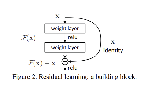
잔차에 더해지는 $\mathbf{x}$ 를 "shortcut connection" 이라 하고 주로 항등 매핑을 사용한다.

# Residual block
def conv3x3(in_planes, out_planes, stride=1, groups=1, dilation=1):
    """3x3 convolution with padding"""
    return nn.Conv2d(in_planes, out_planes, kernel_size=3, stride=stride,
                     padding=dilation, groups=groups, bias=False, dilation=dilation)


def conv1x1(in_planes, out_planes, stride=1):
    """1x1 convolution"""
    return nn.Conv2d(in_planes, out_planes, kernel_size=1, stride=stride, bias=False)


class BasicBlock(nn.Module):
    expansion = 1

    def __init__(self, inplanes, planes, stride=1, downsample=None, groups=1,
                 base_width=64, dilation=1, norm_layer=None):
        super(BasicBlock, self).__init__()
        if norm_layer is None:
            norm_layer = nn.BatchNorm2d
        if groups != 1 or base_width != 64:
            raise ValueError('BasicBlock only supports groups=1 and base_width=64')
        if dilation > 1:
            raise NotImplementedError("Dilation > 1 not supported in BasicBlock")
        # Both self.conv1 and self.downsample layers downsample the input when stride != 1
        self.conv1 = conv3x3(inplanes, planes, stride)
        self.bn1 = norm_layer(planes)
        self.relu = nn.ReLU(inplace=True)
        self.conv2 = conv3x3(planes, planes)
        self.bn2 = norm_layer(planes)
        self.downsample = downsample
        self.stride = stride

    def forward(self, x):
        identity = x

        out = self.conv1(x)
        out = self.bn1(out)
        out = self.relu(out)

        out = self.conv2(out)
        out = self.bn2(out)

        if self.downsample is not None:
            identity = self.downsample(x)

        out += identity
        out = self.relu(out)

        return out

ResNet 주요 개념 및 모델 구조

Identity Mapping by Shortcuts

위에서 설명한 residual learning 의 구조인 Figure 2. 를 도식화하면 다음과 같다.
$\mathbf{y} = \mathcal{F}(\mathbf{x}, \{W_{i}\}) + \mathbf{x} \quad\quad \cdots \quad(1)$

$\mathcal{F}$ 는 residual mapping 을 나타내며 Figure 2. 에서는 두 레이어가 다음과 같은 형태로 있다.
$\mathcal{F} = W_{2}\sigma(W_{1}\mathbf{x}),\quad\quad \sigma : ReLU$

$\mathcal{F} + \mathbf{x}$ 는 shortcut connection 이며, element-wise addition 이다.
단순한 element-wise addition 으로 이루어진 shortcut connection은 학습 파라미터를 늘리거나 계산 복잡도를 늘리지 않는다.

만약 $\mathcal{F} , \mathbf{x}$ 의 차원이 각각 다르다면, linear projection $W_{s}$를 통해 식을 변형할 수 있다.
$\mathbf{y} = \mathcal{F}(\mathbf{x}, \{W_{i}\}) + W_{s}\mathbf{x} \quad\quad \cdots \quad(2)$

물론 (1)의 식에서도 square matrix $W_{s}'$ 를 통해 구조를 변형시켜볼 수 있지만, identity mapping 이 기울기 소실 문제의 해결에서 더 효과적이고 경제적이다. 이후 실험을 통해 확인할 수 있다.

Network Architectures

Residual Network 의 성능 개선을 확인하기 위해 plain/residual nets 를 비교분석하였다.

Plain network

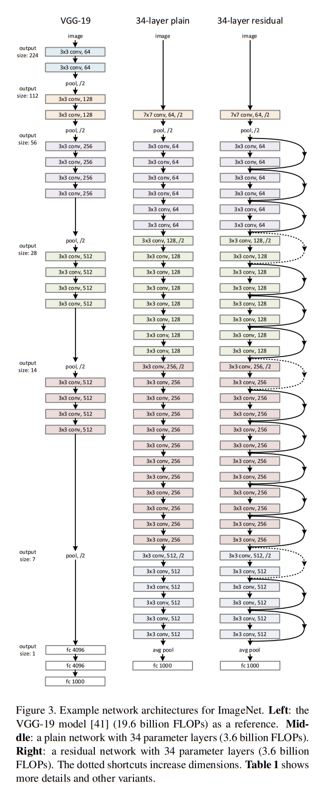
먼저 Figure 3. 의 중앙에 있는 plain baselines network 는 왼쪽의 VGG-19 nets 를 기반으로 만들어졌다. 주로 $3\times3$ 필터의 convolutional layer 들로 이루어져있으며 두 가지 간단한 규칙이 있다.

• for the same output feature map size, same number of filters
• if the feature map size is halved, the number of filters is doubled so as to preserve the time complexity per layer

해당 network 는 weighted layer 가 34개로 34-layer baseline 은 3.6 billioin FLOPs를 가지며 19.6 billion FLOPs 를 가지는 VGG-19 모델의 18% 에 해당된다.

Residual network

다음으로 plain network 에 shortcut connections를 더하여 Residual Network 를 구현한다. input/output 이 같은 차원에서 이루어질 때는 identity shortcut(Eqn.(1)) 을 적용하였고, 차원이 커질 때는 다음의 두 옵션을 정하였다. Figure 3. 의 dotted line shortcuts 가 해당된다.

• (A) : The shortcut still performs identity mapping, with extra zero entries padded for increasing dimensions
• (B) : The projection shortcut in Eqn.(2) is used to match dimensions (1 $\times$ 1 convolutions)
• both option when the shortcuts go across feature maps of two sizes, they are performed with a stride of 2.

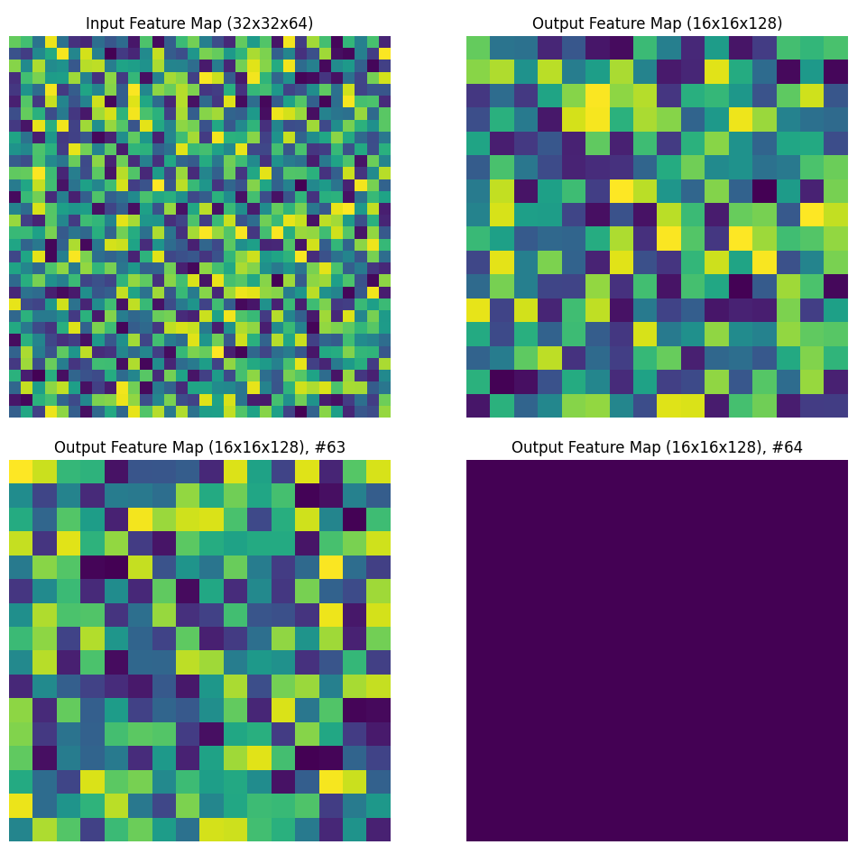
Figure 3. 에 해당되는 dimension 의 증가는 number of feature map 의 증가이며, output shape 은 절반이 된다고 해석하였다. dimension 이 ouput shape 을 가리킬 경우 padding, Eqn.(2) 모두 해당되지 않기 때문이다. 위 해석이 맞을 경우, feature map 의 수가 64에서 128로 증가하고 output shape 이 $32 \times 32$ 에서 $16\times16$ 으로 작아질 때의 예시는 다음과 같다.

Experiments

ImageNet Classification

위 모델들의 성능 비교를 위해 ImageNet 2012가 사용되었으며 해당 데이터셋은 1000 classes, 1.28 million training images, 50k validation images 그리고 100k test images로 이루어져있다.

각 convolution layer 이후, 그리고 activation layer 이전에 batch normalization(BN) 을 추가하였으며 SGD mini-batch size 를 256 개로 정하였다. learning rate 는 0.1 에서 시작하여 10씩 나누면서 진행되었고 학습 과정은 $60 \times 10^4$ 번 반복되었다. 추가로 weight decay 는 0.0001, momentum 은 0.9, dropout은 사용하지 않았다.

Plain network

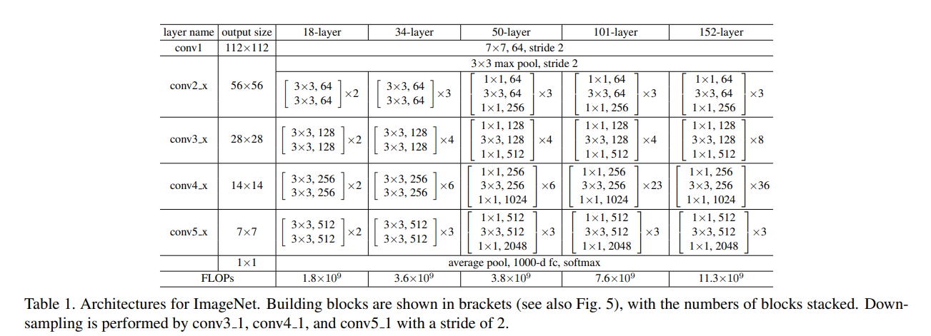
먼저 18-layer 와 34-layer 의 plain network를 비교하였다. Table 1. 을 보면 두 plain network 의 구조는 비슷하며 18-layer network 가 34-layer network 에 포함된 구조라고도 볼 수 있다. 그렇지만 Table 2. 는 Top-1 error 에서 34-layer plain network 가 더 높은 validation error 를 보였음을 나타냈다.

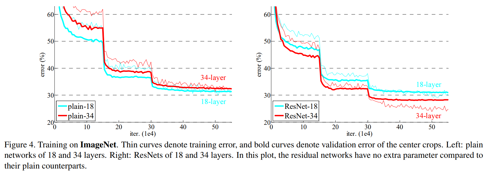
Figure 4. 는 전체 학습 과정의 train/validation error 를 보여주며 validation 뿐 아니라 train error 또한 전체 반복 구간에서 34-layer plain network 가 더 높았음을 알 수 있다. 이때 gradient vanishing 을 의심할 수 있지만 BN layer 가 있어 가중치가 사라지는 문제는 아님을 알 수 있었다. 사실 34-layer network 또한 여전히 나쁘지 않은 성능을 보이기에 solver 의 작동에는 문제가 없었다. 따라서 깊은 plain network 가 지수적으로 낮은 수렴 속도를 가진다고 추측할 수 있었다.

Residual network

다음으로 동일하게 18-, 34-layer plain network 를 기본구조로 두고 각 $3\times 3$ filters 를 가지는 convolution layers 쌍마다 shortcut connection 을 추가한 residual nets(ResNets) 를 평가하였다. shortcut 으로 identity mapping 을 사용하였고 증가한 차원에 대하여 zero-padding 을 적용하였기 때문에 plain network 에 비해 parameter 의 증가는 없었다.

Table 2. 와 Figure 4. 를 따르면 34-layer ResNet 은 18-layer ResNet 보다 validation error 가 약 2.8% 나 적었고, 학습 과정에서도 전반적으로 34-layer ResNet 이 error 가 낮았다. shortcut connections 를 통해 학습률 저하의 문제를 잘 해결하였으며 늘어난 차원을 통해 더 높은 정확도를 얻을 수 있었다.

또한 Table 2. 에 나타나듯 34-layer ResNet 이 plain network 에 비해 top-1 error 에서 3.5% 나 개선되었으며 train error 또한 상당히 줄어들었기에 residual learning 이 deep system 에서 큰 효율성을 가진다고 할 수 있다.

마지막으로 18-layer plain network/ResNet 모두 성능이 좋았고 수렴 속도 면에서 조금의 차이가 있는 것을 볼 수 있다. 18-layer 와 같이 "overly-deep" 하지 않은 network 의 경우 여전히 SGD solver 로 좋은 해답을 구할 수 있음을 알 수 있다.

Deeper Bottleneck Architectures

ImageNet 의 학습 시간 개선의 문제로 더 깊은 network를 소개한다. Figure 5. 의 오른쪽 그림과 같이 병목 구조의 수정된 block 을 Bottleneck architecture 로 정의했다. 기존의 Residual block 에서 사용되던 $3\times3$ filter 의 double convolution layer 는 각각 $1\times1$, $3\times3$, 그리고 $1\times1$ filter 를 가지는 3개의 convolution layer 로 대체되었다.
여기서 $1\times1$ convolution layer 는 입력된 데이터의 차원을 줄여주고, 다시 추출된 데이터의 차원을 늘려주는 역할을 한다.
중간의 $3\times3$ convolution layer 는 작은 차원에서 학습이 일어나므로 계산에 용이한 점을 가진다. 그리고 여기서도 identity shortcut 이 중요한 역할을 한다. 차원이 서로 다른 layer간 연결된 projection shortcut 을 적용할 경우 $1\times1$ layer 의 추가로 계산량이 늘어나게되기 때문에 Bottleneck Architecture 의 장점인 학습 시간 감소를 이끌어내기 위해 identity shortcut 을 사용해야한다.

Figure 5. 의 오른쪽 Bottleneck Architecture 는 ResNet -50/101/152용 building block 을 보여준다.

# Bottleneck block
class Bottleneck(nn.Module):
    # Bottleneck in torchvision places the stride for downsampling at 3x3 convolution(self.conv2)
    # while original implementation places the stride at the first 1x1 convolution(self.conv1)
    # according to "Deep residual learning for image recognition"https://arxiv.org/abs/1512.03385.
    # This variant is also known as ResNet V1.5 and improves accuracy according to
    # https://ngc.nvidia.com/catalog/model-scripts/nvidia:resnet_50_v1_5_for_pytorch.

    expansion = 4

    def __init__(self, inplanes, planes, stride=1, downsample=None, groups=1,
                 base_width=64, dilation=1, norm_layer=None):
        super(Bottleneck, self).__init__()
        if norm_layer is None:
            norm_layer = nn.BatchNorm2d
        width = int(planes * (base_width / 64.)) * groups
        # Both self.conv2 and self.downsample layers downsample the input when stride != 1
        self.conv1 = conv1x1(inplanes, width)
        self.bn1 = norm_layer(width)
        self.conv2 = conv3x3(width, width, stride, groups, dilation)
        self.bn2 = norm_layer(width)
        self.conv3 = conv1x1(width, planes * self.expansion)
        self.bn3 = norm_layer(planes * self.expansion)
        self.relu = nn.ReLU(inplace=True)
        self.downsample = downsample
        self.stride = stride

    def forward(self, x):
        identity = x

        out = self.conv1(x)
        out = self.bn1(out)
        out = self.relu(out)

        out = self.conv2(out)
        out = self.bn2(out)
        out = self.relu(out)

        out = self.conv3(out)
        out = self.bn3(out)

        if self.downsample is not None:
            identity = self.downsample(x)

        out += identity
        out = self.relu(out)

        return out

References

Jiesuck Park, et al. Artificial intelligence–enhanced electrocardiography analysis as a promising tool for predicting obstructive coronary artery disease in patients with stable angina. European Heart Journal - Digital Health (2024) 00, 1–10
Kaiming He, Xiangyu Zhang, Shaoqing Ren, Jian Sun. Deep Residual Learning for Image Recognition arXiv:1512.03385, 2015.
pytorch/resnet.py : https://github.com/pytorch/vision/blob/6db1569c89094cf23f3bc41f79275c45e9fcb3f3/torchvision/models/resnet.py#L124