The most accurate modeling technique for structrued data.

XGBoost는 많은 competition에서 우위를 차지하고 있고, 다양한 dataset에서 최첨단(state-of-art) 결과들을 얻을 수 있다고 함

🧑‍💻Introduction

많은 이 course에서, single decision tree보다 random forest로 prediction을 만들어왔다.
이 과정에서 여러 의사 결정 트리의 예측을 평균화하여 단일 의사 결정 트리보다 더 나은 성능을 달성하는 random forest 방법으로 예측을 수행했다.

우리는 random forest를 "ensemble method" 라고 가리킨다.
ensemble method는 각각 모델의 예측을 섞는 것이다.

여기서는 다른 ensemble method 중 하나인 Gradient Boosting을 배울 것임

Gradient Boosting

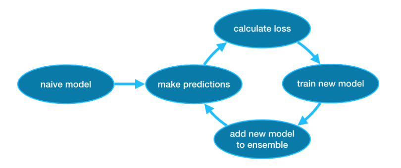
Gradient Boosting은 사이클을 통해 반복적으로 모델을 ensemble에 추가하는 방법이다.
이 것은 예측이 매우 단순(순진)할 수 있는 단일 모델로 ensemble을 initializing 하는 것으로 시작한다. (예측이 부정확하더라도 나중에 ensemble에 추가하면 오류가 해결된다.)

Then, we start the CYCLE!

• 첫번째로, 현재 ensemble을 사용하여 dataset의 각 관측값에 대한 prediction을 생성한다.
  prediction을 만들기 위해서는, ensemble에 있는 모든 모델의 prediction을 추가한다.
• 이 prediction들은 loss function을 계산하는데 사용된다. (MAE 등)
• 그 다음, loss function을 사용하여 ensemble에 추가할 새 모델을 맞춘다. 구체적으로, 이 새 모델을 ensemble에 추가하면 손실이 줄어들도록 model parameter를 결정한다. (참고: Gradient Boosting의 gradient는 loss function의 gradient descent(경사 하강)을 사용하여 이 새 모델의 parameter를 결정한다는 것을 의미)
• 마지막으로, 새 모델을 ensemble에 추가한다.
• 위 과정을 반복한다.
  

Example

import pandas as pd
from sklearn.model_selection import train_test_split

data = pd.read_csv(filepath)

# Select subset of predictors
cols_to_use = ['Rooms', 'Distance', 'Landsize', 'BuildingArea', 'YearBuilt']
X = data[cols_to_use]

# Select target
y = data.Price

# Seperate data into training and validation sets
X_train, X_valid, y_train, y_valid = train_test_split(X, y)

이 예제에서는 XGBoost 라이브러리로 작업한다.
XGBoost : Extreme Gradient Boosting
성능과 속도에 중점을 둔 몇가지 추가 기능을 갖춘 Gradient Boosting을 구현한 것
(scikit-learn에 다양한 gradient boosting이 있지만 XGBoost가 몇가지 이점이 있음)

from xgboost import XGBRegressor

my_model = XGBRegressor()
my_model.fit(X_train, y_train)

prediction & evaluate

from sklearn.metrics import mean_absolute_error

predictions = my_model.predict(X_valid)
print("Mean Absolute Error :" + str(mean_absolute_error(predictions, y_valid))

Parameter Tuning

XGBoost에는 정확도와 훈련 속도에 큰 영향을 줄 수 있는 몇 가지 매개변수가 있다.

n_estimators

n_estimators
모델링 주기를 몇 번 거칠 것인지 정하는 parameter
= 앙상블에 포함되는 모델의 수

• 값이 너무 작으면 Underfitting이 발생, train/test 데이터에서 예측이 부정확
• 값이 너무 높으면 Overfitting이 발생, test에 대한 예측이 부정확

일반적인 값의범위는 100 ~ 1,000인데, 아래에서 설명할 learning_rate에 따라 크게 달라진다.

다음은 ensemble의 model 수를 설정하는 코드

my_model = XGBRegressor(n_estimators=500)
my_model.fit(X_train, y_train)

early_stopping_rounds

early_stopping_rounds
n_estimators에 이상적인 값을 자동으로 찾는 방법을 제공
hard stop이 아니더라도 validation이 개선되지 않으면 모델 반복을 중단함

n_estimators의 값을 높게 설정하고 early_stopping_rounds를 사용하여 최적의 중단 시점을 찾는 것이 현명하다고 함

어떤 무작위적인 확률로 validation이 개선되지 않는 round가 있을 수 있으므로 early_stopping_rounds를 5로 설정하는 것이 합리적임
-> 5번 연속 저하될 시 중지

early stop을 사용할 경우 validation score 계산을 위한 일부 데이터도 따로 설정해야 한다. 이는 eval_set parameter를 사용하여 수행

다음은 예시

my_model = XGBRegressor(n_estimators=500)
my_model.fit(X_train, y_train,
		     early_stopping_rounds=5,
             eval_set=[(X_valid, y_valid)],
             verbose=False)

verbose는 정보 상세 출력 옵션

learning_rate

각 구성 요소 모델의 prediction을 단순히 합산하여 예측을 얻는 대신, 각 모델의 predictiond에 작은 숫자(learning_rate, 학습률)를 곱한 후 합산할 수 있다.

즉, ensemble에 추가하는 각 tree가 더 적게 기여한다는 뜻.
-> Overfitting 없이 n_estimators의 값을 더 높게 설정할 수 있다.
early stop을 사용하면 적절한 트리 수가 자동으로 결정된다.

일반적으로 learning rate가 적고, n_estimators가 클수록 더 정확한 XGBoost 모델을 얻는다.
하지만 주기 동안 더 많은 반복을 수행하므로 모델 학습에 시간이 더 오래 걸린다.
기본적으로 XGBoost는 learning_rate를 0.1로 설정한다.

예시

my_model = XGBRegressor(n_estimators=1000, learning_rate=0.05)
my_model.fit(X_train, y_train,
			 early_stopping_rounds=5,
             eval_set=[(X_valid,  y_valid)],
             verbose=False)

n_jobs

run time을 고려해야하는 대규모 dataset에는 병렬처리 (parallelism)를 사용하여 모델을 더 빠르게 빌드할 수 있다.
n_jobs parameter를 사용하여 컴퓨터의 코어 수와 동일하게 설정한다.
(작은 dataset은 할 필요 X)

my_model = XGBRegressor(n_estimators=1000, learning_rate=0.05, n_jobs=4)
my_model.fit(X_train, y_trainm
			 early_stopping_rounds=5,
             eval_set=[(X_valid, y_valid)],
             verbose=False)

Conclusion

XGBoost는, 이미지나 동영상 같은 이색적 데이터와 달리 pandas 같은 표 형식의 데이터에 적합한 라이브러리. parameter tuning을 적극적으로 하자.