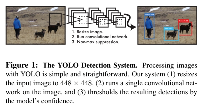
안녕하세요! 오늘은 당시 two stage Object Detection 모델이 성행할 때 혜성같이 single netowork detection 모델로 등장해 지금까지 다양한 버전이 발전되어 온 YOLO(You Only Look Once)모델에 대해서 살펴보겠습니다. 이 모델은 이름에서도 알 수 있다시피 기존의 Faster R-CNN과 같이 Region proposal과 Detection model을 각각 학습해야하는 모델들과 달리 region proposal과 Detection을 하나의 pipeline으로 학습하여 이미지를 처리하는 속도를 매우 단축시켜 real time detection의 시작을 알렸습니다.

Paper Review

본 논문의 저자는 R-CNN 기반의 모델들의 복잡한 구조에 대한 문제점을 해결하고자 하였습니다. 특히 region proposal 방법으로 potential box들을 생성하고, 이것을 objectness에따라 분류하고, 다시 detection하고 하는 등 여러 과정들을 거치다보니 학습도 오래걸리고 optimize도 쉽지 않았습니다. 그래서 이에 대한 부분을 해결하고자 single regression detection model을 개발하였고, image pixel 단계에서 바로 bounding box coordinate와 class probability를 예측하는 모델인 YOLO를 제안하게 되었습니다.

저자는 YOLO를 제안하면서 3가지 장점을 설명했습니다.

1. complex pipeline에서 벗어나 매우 빠른 detection 속도를 구사합니다.
2. image 전체를 이용해 학습하기 때문에 *image를 global하게 추론합니다.
3. 다양한 object의 representation에 generalize되어 있어 새로운 domain이나 다양한 input에 대해 적용이 가능합니다.

YOLO의 특징에 대해 알아보았으니 Model Architecture 구조를 알아보겠습니다.

Unified Detection

논문에서 모델의 Architecture를 설명하면서 Unified라는 표현을 썼을만큼 저자는 기존에 **Detection model architecture에 분리되어 있던 요소들을 하나의 Network에 모두 포함**하였다는 것을 강조하고자 합니다. image로부터 feature들을 추출하고, 전체 이미지의 모든 부분에 bounding box를 생성해 각 box마다 모든 class에 대한 예측하는 과정을 모두 포함합니다. 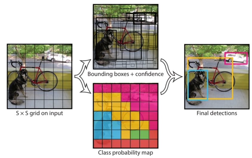YOLO는 위 그림에서 볼 수 있다시피 input image에 Convolution Network를 이용해 S*S Feature map 즉 **S*S의 Grid를 생성**합니다. 그리고 **각 Grid 별로 Bounding box Regression과 classification 연산을 통해 Object Detection**을 하게 됩니다.

Network Design

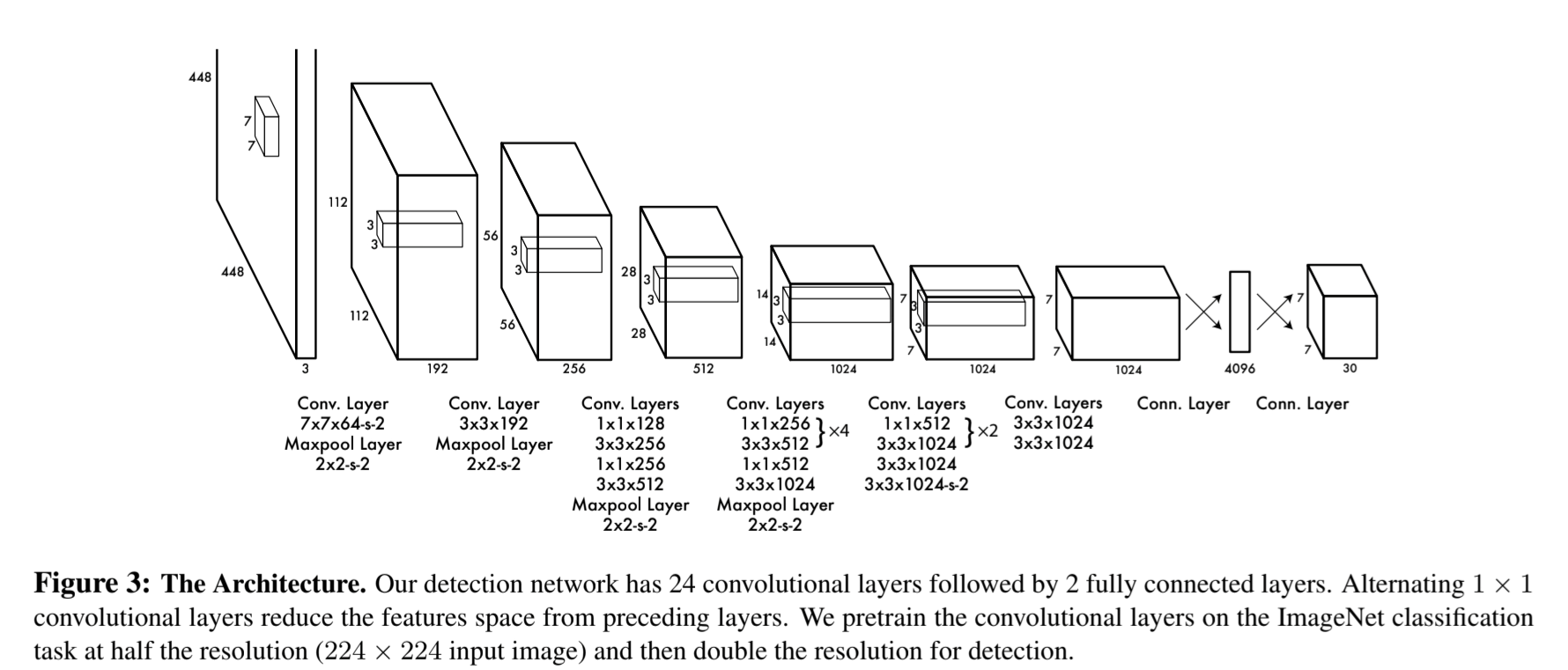YOLO의 전체적인 Architecture는 GoogLeNet에서 영감을 받았다고 합니다. 448*448 size의 image input에 conv-layer 연산을 통해 S*S grid를 갖는 Feature map을 추출하고, 두 번의 Fully-Connected layer를 통해 최종 예측값을 도출해 낼 수 있습니다.

Final Output

Network Design의 Archtecture를 보면 마지막 output이 7*7*30 tensor의 형태를 띠고 있습니다. 이것은 YOLO가 single network를 구축하면서 각 grid(S=7)별로 필요한 prediction이 30개 라는 것을 의미합니다.
YOLO는 각 grid 별로 크게 3가지(Bounding box, Confidence, Class)를 예측합니다.

1. Bounding box

• 논문에서는 Bounding box와 Confidence 연산은 같이 연관지어 설명합니다. Bounding Box는 grid별로 B개를 예측하는데, 각 box는 (x,y,h,w) 4개의 값으로 특정이 되며, x,y는 해당 grid cell에 Normalize된 box의 center 좌표이고, h,w는 image size에 따라 Normalize 된 값으로 나타냅니다.

2. Confidence

• Confidence는 Objectness와 비슷한 개념으로 box에 object가 있는지 여부와 그 box의 위치가 실제 object와 비교해서 얼마나 정확한지를 포함하는 개념입니다. 논문에서는 $Pr(Object)*IOU^{truth}_{pred}$로 제안합니다. 만약 해당 cell에 object가 없다면 confidence score는 0이 됩니다.

3. Class probability

• 해당 grid cell에 object가 있다는 가정 하에 어떤 class인지를 예측하는 과정으로 논문에서는 $Pr(Class_i|Object)$로 제안합니다.
• 다만 각 grid cell에 B개의 Box를 예측했던 것과 달리 Class는 grid 당 1개만 에측하게 되며, test시에는 IOU값의 영향을 받아 class-specific confidence score를 예측하게 됩니다.

각 grid cell에서 B개의 bounding box를 예측하고, C개의 class probability를 예측한다고 했을 때 한 cell 당 $B*(4+1)+C$개의 prediction이 필요하고, 한 image당 S*S의 grid cell을 가지기 때문에

Training

Darknet Pre-train
논문에서는 위 architecture 중 처음 20개의 conv-layer(Darknet)를 pre-training에 활용했습니다. 이후 Detection을 위해 4개의 conv-layer와 2개의 FC-layer를 더해 지금의 Architecture가 되었다고 설명합니다.

Activation
저자는 마지막 layer를 제외하고 학습에 활용될 Activation 함수는 Leaky ReLU를 제안합니다.

Loss Function
논문에서 제안하는 Loss Function은 각 prediction 별로 sum-squared error 연산을 통해 전체 Loss를 계산합니다.

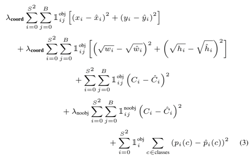
Loss Function은 grid cell에 object가 포함하고 있는지 여부에 따라 가중치 λ를 부여하였고, 하나의 bounding box가 1개의 object만을 예측하는데 집중할 수 있도록 $1^{obj}_{ij}$를 통해 responsible을 부여했습니다.

Others

• Dataset: PASCAL VOC
• batchsize: 64
• momentum: 0.9
• weight_decay: 0.0005
• dropout: 첫번째 fc-layer이후 0.5 적용
• data augmentation: random scaling, HSV color space에 exposure, saturation 조절

Code Review

전체적인 코드는 Github에 올려놓겠습니다. 본 포스트에는 위 paper review에 설명된 주요 알고리즘에 대해서 설명하겠습니다.

YOLO를 구현하는 전체적인 순서는 다음과 같습니다.

1. Modeling
2. Loss Function
3. Dataset
4. Training
5. Predict

Modeling

YOLO 모델은 24개의 Conv-layer와 2개의 FC-layer로 이루어져 있습니다. 코드로 구현한 Conv-layer는 BatchNormalization과 Leaky-ReLU를 적용한 Conv-Block을 먼저 구현한 뒤, 이 Block들을 Architecture에 맞게 쌓아주었습니다.

Architecture 구현에 필요한 config

architecture_config = [
    (7, 64, 2, 3),
    "M",
    (3, 192, 1, 1),
    "M",
    (1, 128, 1, 0),
    (3, 256, 1, 1),
    (1, 256, 1, 0),
    (3, 512, 1, 1),
    "M",
    [(1, 256, 1, 0), (3, 512, 1, 1), 4],
    (1, 512, 1, 0),
    (3, 1024, 1, 1),
    "M",
    [(1, 512, 1, 0), (3, 1024, 1, 1), 2],
    (3, 1024, 1, 1),
    (3, 1024, 2, 1),
    (3, 1024, 1, 1),
    (3, 1024, 1, 1),
]

Conv Block

class conv_block(nn.Module):
    
    def __init__(self,in_channels,out_channels,**kwargs):
        super(conv_block,self).__init__()
        self.conv = nn.Conv2d(in_channels,out_channels,bias=False,**kwargs,)
        self.bn = nn.BatchNorm2d(out_channels)
        self.leaky_relu = nn.LeakyReLU(0.1)
    
    def forward(self,x):
        x = self.leaky_relu(self.bn(self.conv(x)))
        return x

YOLO Architecture

class Yolov1(nn.Module):
    def __init__(self,config,in_channels=3,**kwargs):
        super(Yolov1,self).__init__()

        self.config = config
        self.in_channels = in_channels
        self.darknet = self.create_conv_layers(self.in_channels)
        self.fcnet = self.create_fc_layers(**kwargs)
        
    def create_conv_layers(self,in_channels):
        conv_layers=[]
        for x in self.config:
            if x == "M":
                conv_layers.append(nn.MaxPool2d(kernel_size=2,stride=2))
            elif type(x) == list:
                for i in range(x[-1]):
                    conv_layers.append(conv_block(in_channels,x[0][1],kernel_size=x[0][0],stride=x[0][2],padding=x[0][3]))
                    conv_layers.append(conv_block(x[0][1],x[1][1],kernel_size=x[1][0],stride=x[1][2],padding=x[1][3]))
                    in_channels = x[1][1]
            else:
                conv_layers.append(conv_block(in_channels,x[1],kernel_size=x[0],stride=x[2],padding=x[3]))
                in_channels = x[1]
        return nn.Sequential(*conv_layers)

    def create_fc_layers(self,split_size,num_boxes,num_classes):
        s,b,c = split_size,num_boxes,num_classes
        fc_layers=nn.Sequential(
            nn.Flatten(),
            nn.Linear(s*s*1024,4096),
            nn.Dropout(0.5),
            nn.LeakyReLU(0.1),
            nn.Linear(4096,s*s*(5*b+c))
        )
        return fc_layers

    def forward(self,x):
        x1 = torch.flatten(self.darknet(x),start_dim = 1)
        x2 = self.fcnet(x1)
        return x2

위 코드에서 Darknet을 비롯한 Conv-layer를 먼저 구현하고, 이를 Flatten 한 뒤, FC-layer를 적용하였습니다. 논문에서 grid cell=7*7, bounding box=2, class=20으로 제안하였기 때문에 output tensor는 7*7*30의 size를 갖습니다.

Loss Function

loss function은 논문 리뷰에서 다뤘듯 sum-squared error을 이용하였으며, object여부에 따라 가중치를 조절해 적용하였습니다. 이 과정에서는 저자가 bounding box에 "responsible"을 주기 위해 활용한 $1^{obj}_{ij}$에 대한 구현과 각기 다른 prediction 값을 flatten하고 연산하는 과정에서 output dimenstion을 맞추는 과정에서 조금 복잡함이 있었습니다.

class YoloLoss(nn.Module):
    def __init__(self):
        super(YoloLoss,self).__init__()
        self.lambda_coord = 5
        self.lambda_noobj = 0.5
        self.mse = nn.MSELoss(reduction="sum")
        
    def forward(self, p, t):
        p = p.reshape(-1,7,7,20+5*2)
        t_box = t[...,21:25]
        pred_box1,pred_box2 = p[...,21:25],p[...,26:30]
        pred_conf1,pred_conf2 = p[...,20].unsqueeze(-1),p[...,25].unsqueeze(-1)

        iou1 = IOU(pred_box1,t_box)
        iou2 = IOU(pred_box2,t_box)

        ious = torch.cat([iou1.unsqueeze(0),iou2.unsqueeze(0)],dim=0)
        iou_max_val, best_bbox = torch.max(ious, dim = 0) #max ious value, max ious box

        actual_obj = t[...,20].unsqueeze(-1)
        
        box_target = actual_obj*t_box
        box_target[...,2:] = torch.sqrt(box_target[...,2:]) #w,h는 loss에서 sqrt가 들어가야함.

        box_pred = actual_obj*(best_bbox*pred_box2 + (1-best_bbox)*pred_box1)
        box_pred[...,2:] = torch.sign(box_pred[...,2:]) * torch.sqrt(torch.abs(box_pred[...,2:]+1e-6))

        box_coord_loss = self.mse(
            torch.flatten(box_pred,end_dim=-2),
            torch.flatten(box_target,end_dim=-2)
        )

        conf_pred = actual_obj*(best_bbox*pred_conf2 + (1-best_bbox)*pred_conf1)
        
        obj_loss = self.mse(
            torch.flatten(conf_pred),
            torch.flatten(actual_obj)
        )

        #no object loss
        no_obj_loss = self.mse(
            torch.flatten((1 - actual_obj) * pred_conf1,start_dim = 1),
            torch.flatten((1 - actual_obj) * actual_obj,start_dim = 1)
        )
        
        no_obj_loss2 = self.mse(
            torch.flatten((1 - actual_obj) * pred_conf2,start_dim = 1),
            torch.flatten((1 - actual_obj) * actual_obj,start_dim = 1)
        )
        
        #class loss
        class_loss = self.mse(
            torch.flatten(actual_obj * p[..., :20],end_dim = -2),
            torch.flatten(actual_obj * t[..., :20],end_dim = -2)
        )
        
        loss = (
            self.lambda_coord * box_coord_loss +
            obj_loss +
            self.lambda_noobj * (no_obj_loss2 + no_obj_loss) +
            class_loss
        )
        
        return loss

Dataset

Dataset은 Kaggle에 있는 'PascalVOC_YOLO'를 활용하였다. 본 데이터셋은 train,test에 대한 index 정보가 csv형태로 담겨 있습니다. image는 Darknet의 input size인 448*448로 변형시켜주었고, label에서 (x,y,h,w) 정보는 논문에서 설명한대로 grid cell과 image size에 맞게 Normalize해주었습니다.

class custom_dataset(Dataset):
    def __init__(self,path,s=7,mode='train',transformation = True,device=device):
        super(custom_dataset,self).__init__()
        self.path = path
        self.mode = mode
        self.s = s
        self.transformation = transformation
        self.device = device

        train_index = pd.read_csv(self.path + '/train.csv',header=None)[:500]
        train_index.columns = ['image','label']
        test_index = pd.read_csv(self.path + '/test.csv',header=None)[:30]
        test_index.columns = ['image','label']
        self.train_index = train_index
        self.test_index = test_index

    def load_data(self,label_path):
        labels = []
        boxes = []
        with open(label_path, 'r') as file:
            lines = file.readlines()
            for line in lines:
                res = line.strip().split(' ')
                labels.append(res[0])
                boxes.append([float(i) for i in [res[1],res[2],res[3],res[4]]])
        return labels, boxes

    def make_target(self, labels, boxes):
        split = self.s
        target = np.zeros((split,split,20+5))
    
        for n in range(len(labels)):
            i,j = int(boxes[n][0]*split),int(boxes[n][1]*split)
            box_coord = [boxes[n][0]*split-i,boxes[n][1]*split-j,boxes[n][2]*split,boxes[n][3]*split]
            target[i,j,int(labels[n])-1]=1
            target[i,j,-5] = 1
            target[i,j,-4:] = box_coord
            
        target = torch.tensor(target).to(self.device)
        return target

    def transformer(self,img):
        mytrans = transform.Compose([
                transform.Resize((448,448)),
                transform.ToTensor(),
            ])
        if self.transformation:
            return mytrans(img)
        else:
            return img
        
    
    def __getitem__(self,index):
        if self.mode == 'train':
            image_path = self.path + '/images/'+ self.train_index['image'][index]
            label_path = self.path + '/labels/'+ self.train_index['label'][index]
            
        elif self.mode == 'test':
            image_path = self.path + '/images/'+ self.test_index['image'][index]
            label_path = self.path + '/labels/'+ self.test_index['label'][index]
        
        l,b = self.load_data(label_path)
        t = self.make_target(l,b)
        img = Image.open(image_path).convert("RGB")
        img = self.transformer(img)
        img = img.to(self.device)
        return img,t

            
    def __len__(self):
        if self.mode == 'train':
            return len(self.train_index['image'])
        elif self.mode == 'test':
            return len(self.test_index['image'])

논문에서는 학습 시에 Data Augmentation을 적용하였지만 본 코드 작성 시에는 제외하였습니다.

Training

논문에서 제안한 hyperparameter를 활용해 model을 학습한다. 실제로 training 단계에서는 Darknet도 pretrain 되지 않았기 때문에 성능이 좋지는 않았다.

Train hyperparameter

seed = 123
torch.manual_seed(seed)

num_epochs = 10
batch = 64

w8_decay = 0
optimizer = torch.optim.SGD(model.parameters(), lr = 2e-5, momentum = 0.9, weight_decay = 0.0005)

#loss
lossfn = YoloLoss()

#model
model = Yolov1(architecture_config, split_size=7, num_boxes=2, num_classes=20).to(device)

Training

def train(loader=train_loader):

    for epoch in range(num_epochs):
        loop = tqdm(loader, leave=True)
        mean_loss=[]
        loss=0
        for b_id, (x,y) in enumerate(loop):
            optimizer.zero_grad()
            pred = model(x)
            loss = lossfn(pred,y)
            loss.backward()
            optimizer.step()
            
            l = loss.item()
            mean_loss.append(l)
            loop.set_postfix(loss = l)
            
        print(f"Mean loss was {sum(mean_loss)/len(mean_loss)}")

Test

def test(loader=test_loader):
    loop = tqdm(loader,leave=True)
    mean_loss=[]
    with torch.no_grad():
        for b_id, (x,y) in enumerate(loop):
            pred = model(x)
            loss = lossfn(pred,y)
            l = loss.item()
            mean_loss.append(l)
    print(f"Mean loss was {sum(mean_loss)/len(mean_loss)}")

Predict

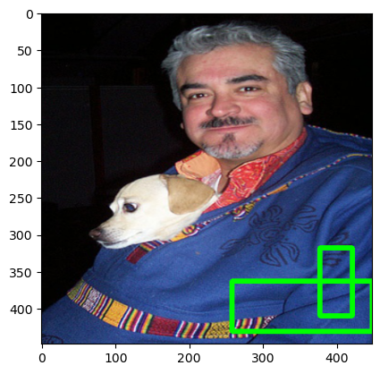
Model을 통해 Object Detection 과정에서 활용한 Utility 함수 및 결과입니다.

Utils

1. model의 예측 값이 7*7*30 tensor이기 때문에 이를 class, confident, box 로 다시 나눠주는 함수입니다.

    def convert_pred(output):
    p = output.reshape(-1,7,7,20+5*2)
    pred_box1,pred_box2 = p[...,21:25],p[...,26:30]
    pred_conf1,pred_conf2 = p[...,20].permute(1,2,0),p[...,25].permute(1,2,0)
    pred_class = p[...,:20]

    scores = torch.cat([pred_conf1.unsqueeze(0),pred_conf2.unsqueeze(0)],dim=0)
    best_box = scores.argmax(0).unsqueeze(0)
    
    best_boxes = best_box*pred_box2 + (1-best_box)*pred_box1
    best_confs = best_box*pred_conf2 + (1-best_box)*pred_conf1
    best_class = pred_class.argmax(-1).unsqueeze(-1)

    convert_preds = torch.cat(
        [best_class,best_confs,best_boxes],dim=-1
    )
    return convert_preds

2. model에서 예측한 box들은 grid cell과 image에 대해 Normalize되어 있기 때문에 이를 다시 원래 size로 변환시켜줍니다.

 def pred_to_box(boxes,size = 448):
    for i,j in zip(range(boxes.shape[1]),range(boxes.shape[2])):
        x1 = size/boxes.shape[1]*i+boxes[...,0]-size*boxes[...,2]/2
        x2 = size/boxes.shape[1]*i+boxes[...,0]+size*boxes[...,2]/2
        y1 = size/boxes.shape[2]*j+boxes[...,1]-size*boxes[...,3]/2
        y2 = size/boxes.shape[2]*j+boxes[...,1]+size*boxes[...,3]/2
        xyxy = torch.cat([x1,x2,y1,y2],dim=0).permute(1,2,0)
        xyxy = torch.clip(xyxy,0,448)
    return pred_to_box

3. 각 Grid 별로 예측한 Bounding box에 대해 NMS를 적용하고 최종 Detection된 box를 그려줍니다.

def nms(boxes, probs, threshold, iou_threshold):
    boxes = torch.flatten(boxes,end_dim=-2)
    probs = torch.flatten(probs)
    # 내림차순으로 정렬
    order = probs.argsort().cpu().data.numpy()

    # 개수 대로 true 리스트 생성
    keep = [True]*len(order)
 
  
    for i in range(len(order)-1):
        if probs[i]<threshold:
            keep[i]=False

        for j, ov in enumerate(boxes[order[i+1:]]):
            iou = IOU(ov,boxes[order[i]])
            if iou > iou_threshold:
            # IOU가 특정 threshold 이상인 box를 False로 세팅
                keep[order[j+i+1]] = False
    return keep

최종 Detection 된 결과는 다음과 같습니다. 학습이 잘 되지 않았기 때문에 좋은 결과는 아니지만 그래도 논문하나를 처음부터 끝까지 구현해서 결과 값까지 도출해본 것이 큰 경험이 될 것이라 생각합니다.