Python
Numpy
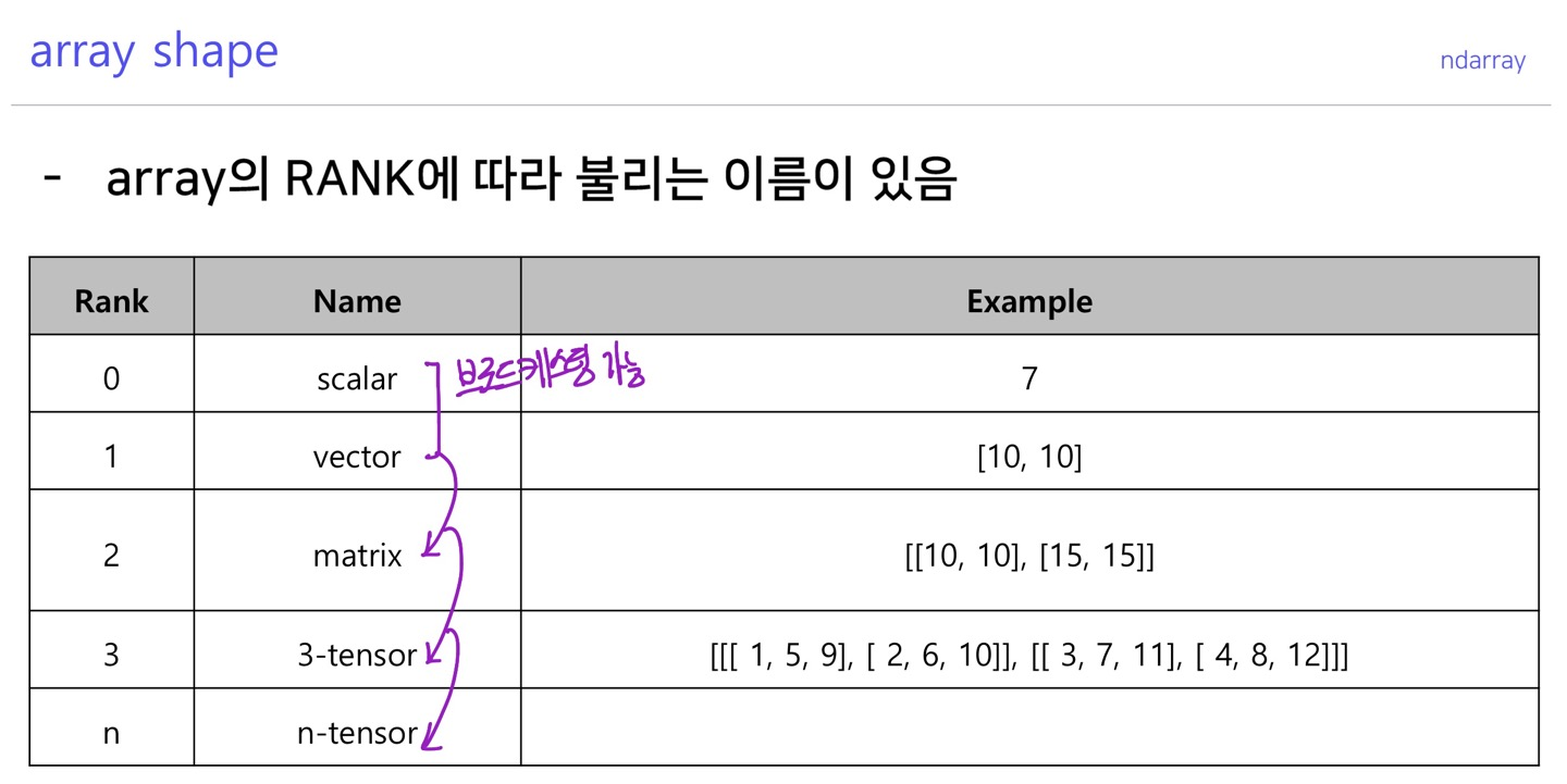
array shape
Handling shape
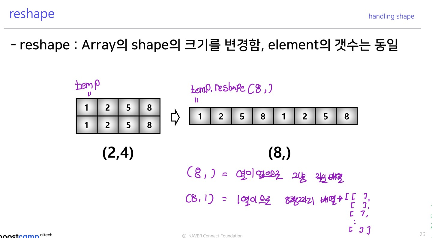
reshape
>>> temp=np.array([[[1,2,3,4],[5,6,7,8]],[[9,10,11,12],[13,14,15,16]]])
>>> temp
array([[[ 1,  2,  3,  4],
        [ 5,  6,  7,  8]],

       [[ 9, 10, 11, 12],
        [13, 14, 15, 16]]])
>>> temp.reshape(16,)
array([ 1,  2,  3,  4,  5,  6,  7,  8,  9, 10, 11, 12, 13, 14, 15, 16])
>>>
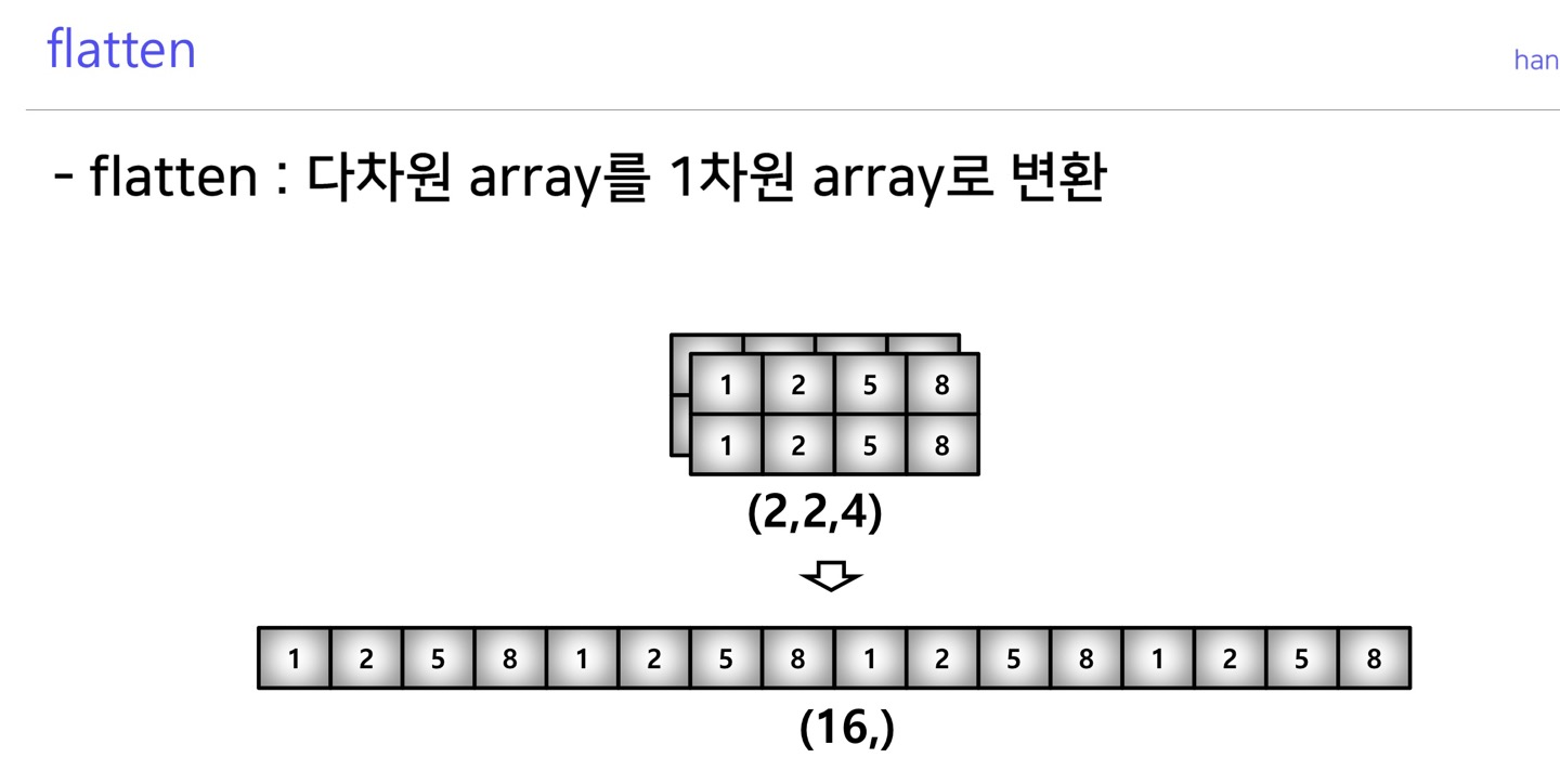
flatten
>>> temp=np.array([[[1,2,3,4],[5,6,7,8]],[[9,10,11,12],[13,14,15,16]]])
>>> temp
array([[[ 1, 2, 3, 4],
[ 5, 6, 7, 8]],
[[ 9, 10, 11, 12],
[13, 14, 15, 16]]])
>>> temp.flatten()
array([ 1, 2, 3, 4, 5, 6, 7, 8, 9, 10, 11, 12, 13, 14, 15, 16])
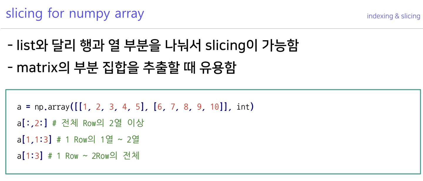
>>>slicing
>>> temp
array([[[ 1,  2,  3,  4],
        [ 5,  6,  7,  8]],

       [[ 9, 10, 11, 12],
        [13, 14, 15, 16]]])
>>> temp.shape
(2, 2, 4)

#슬라이싱의 범위가 표기되어 있지 않은 경우 idx로 생각함
>>> temp[:,1,:]
array([[ 5,  6,  7,  8],
       [13, 14, 15, 16]])

#슬라이싱의 범위는 [시작:끝):간격] 이다. 범위지정을 하지 않은 경우 전체가 포함
>>> temp[:,0:1,:]
array([[[ 1,  2,  3,  4]],

       [[ 9, 10, 11, 12]]])
>>>
Creation function
arange
>>> np.arange(30)
array([ 0,  1,  2,  3,  4,  5,  6,  7,  8,  9, 10, 11, 12, 13, 14, 15, 16,
       17, 18, 19, 20, 21, 22, 23, 24, 25, 26, 27, 28, 29])
#arange(시작,끝(미포함),간격)
>>> np.arange(0,30,5)
array([ 0,  5, 10, 15, 20, 25])
>>> np.arange(30).reshape(5,6)
array([[ 0,  1,  2,  3,  4,  5],
       [ 6,  7,  8,  9, 10, 11],
       [12, 13, 14, 15, 16, 17],
       [18, 19, 20, 21, 22, 23],
       [24, 25, 26, 27, 28, 29]])
>>>
array의 범위를 지정하여 list를 생성하는 numpy 명령어
ones, zeros, empty
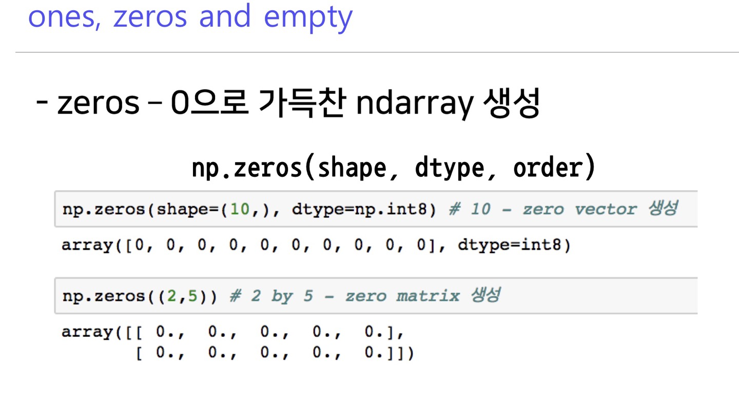
zeros : 0으로 만든 array 생성
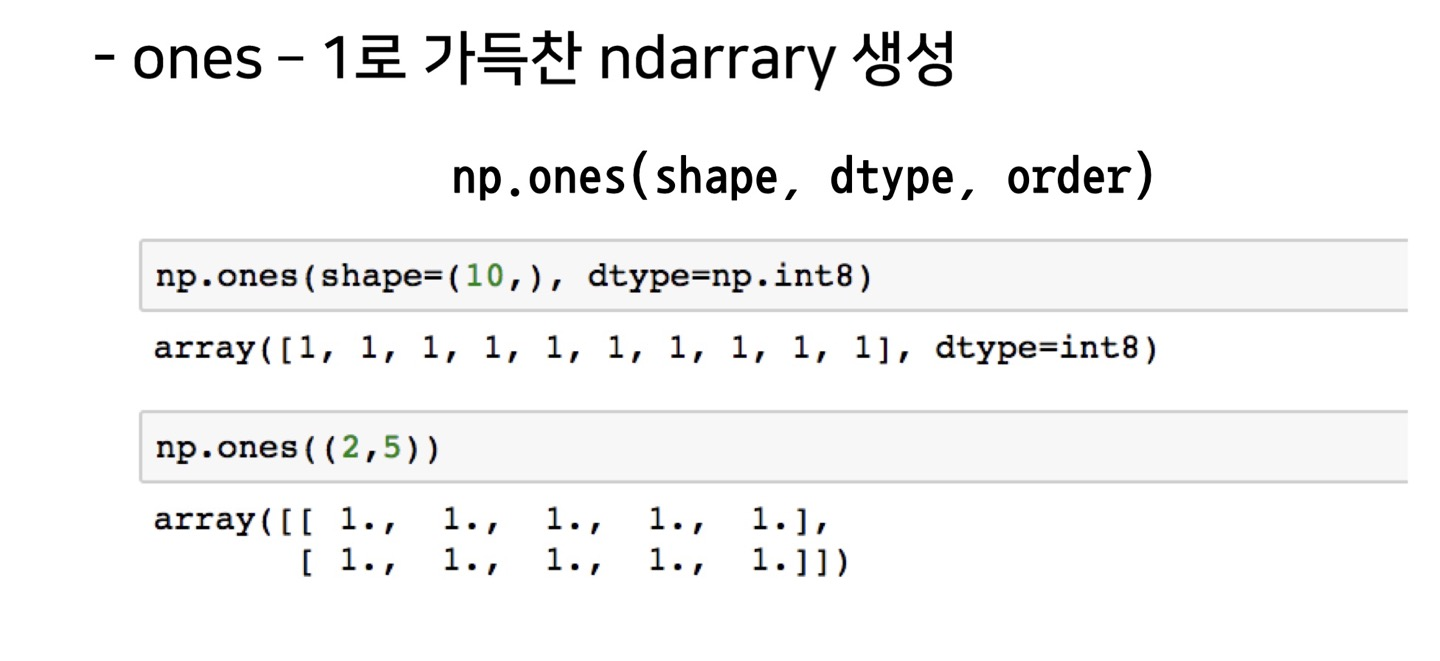
ones : 1로 만든 array 생성
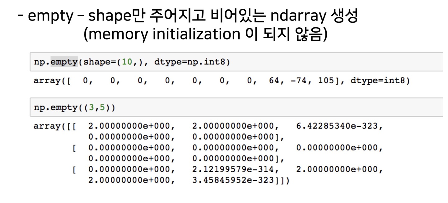
empty : 비어있는 array 생성
something(ones, zeros, empty)_like
>>> temp
array([[[ 1,  2,  3,  4],
        [ 5,  6,  7,  8]],

       [[ 9, 10, 11, 12],
        [13, 14, 15, 16]]])
>>> np.ones_like(temp)
array([[[1, 1, 1, 1],
        [1, 1, 1, 1]],

       [[1, 1, 1, 1],
        [1, 1, 1, 1]]])
>>> np.zeros_like(temp)
array([[[0, 0, 0, 0],
        [0, 0, 0, 0]],

       [[0, 0, 0, 0],
        [0, 0, 0, 0]]])
>>>
기존의 narray shape 모양의 ones, zeros, empty 행렬을 생성
identity
>>> np.identity(n=3)
array([[1., 0., 0.],
       [0., 1., 0.],
       [0., 0., 1.]])
>>>
nxn단위행렬을 생성
eye
>>> np.eye(3,5)
array([[1., 0., 0., 0., 0.],
       [0., 1., 0., 0., 0.],
       [0., 0., 1., 0., 0.]])
>>> np.eye(3,5,k=1)
array([[0., 1., 0., 0., 0.],
       [0., 0., 1., 0., 0.],
       [0., 0., 0., 1., 0.]])
>>>
nxm행렬에서 대각선의 성분이 1인 행렬을 생성(1의 시작 인덱스를 k=값으로 변경시킬 수 있다)
diag
>>> temp
#diag은 3차원 이상의 tensor에서는 적용이 안됨
array([[[ 1,  2,  3,  4],
        [ 5,  6,  7,  8]],

       [[ 9, 10, 11, 12],
        [13, 14, 15, 16]]])
>>> np.diag(temp)
Traceback (most recent call last):
    raise ValueError("Input must be 1- or 2-d.")
ValueError: Input must be 1- or 2-d.
>>> temp2=np.arange(9).reshape(3,3)
>>> temp2
array([[0, 1, 2],
       [3, 4, 5],
       [6, 7, 8]])
>>> np.diag(temp2)
array([0, 4, 8])
#k값으로 시작 인덱스를 변경할 수 있음
>>> np.diag(temp2,k=1)
array([1, 5])
>>>
대각행렬의 값을 추출
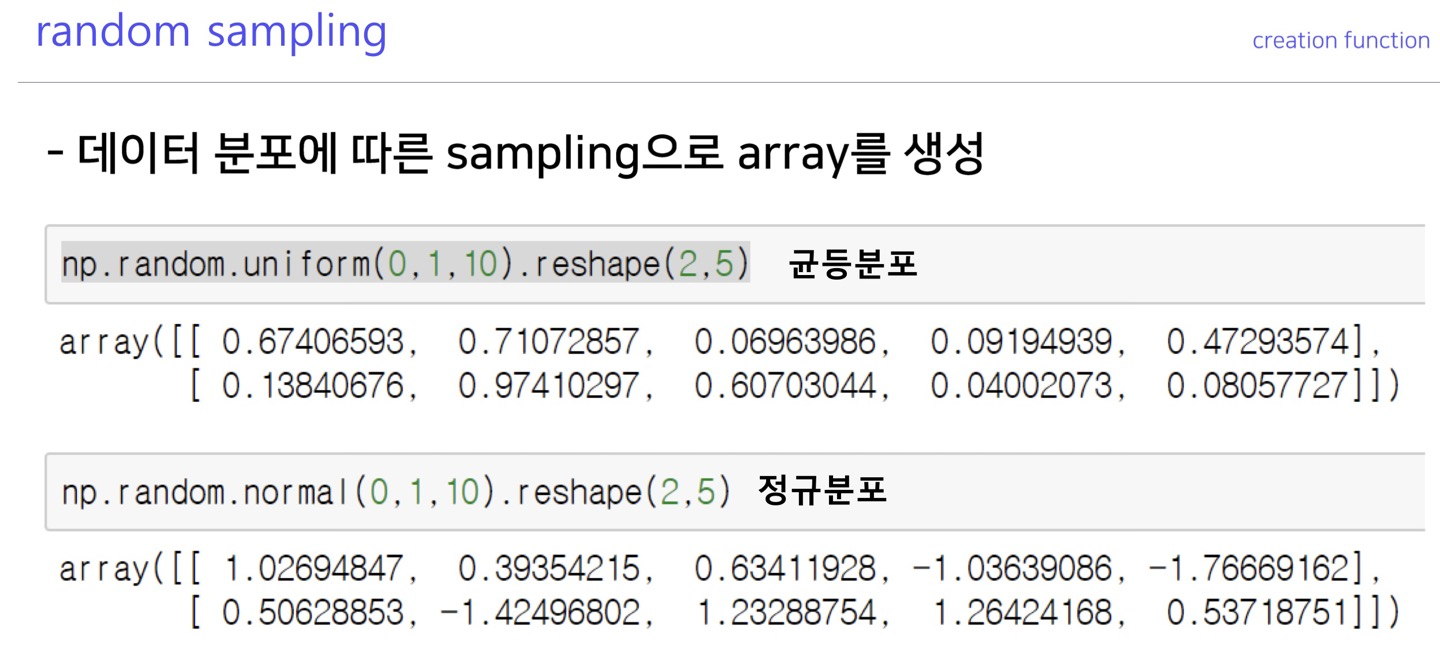
random sampling
Operation functions
axis
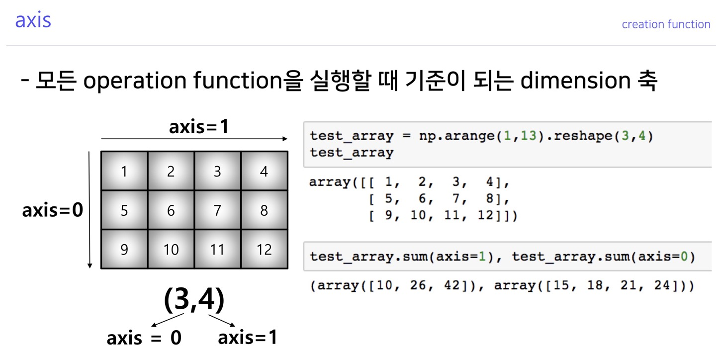
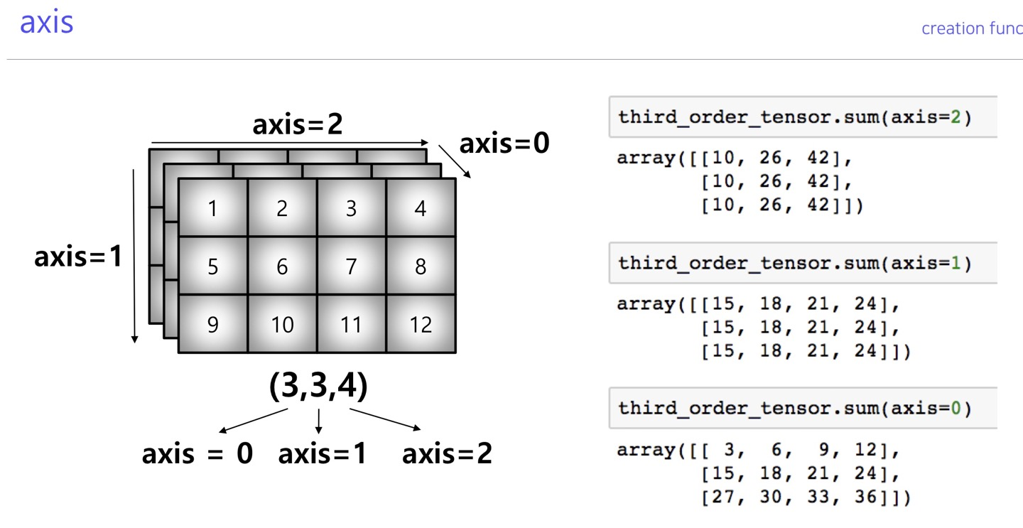
넘파이에서 재공하는 모든 연산의 기준이 되는 축을 결정하는 요소
n tensor가 (a,b,c...) 이면 a부터 순서대로 a : axis=0, b : axis=1, c : axis=2 이다.
mean, std
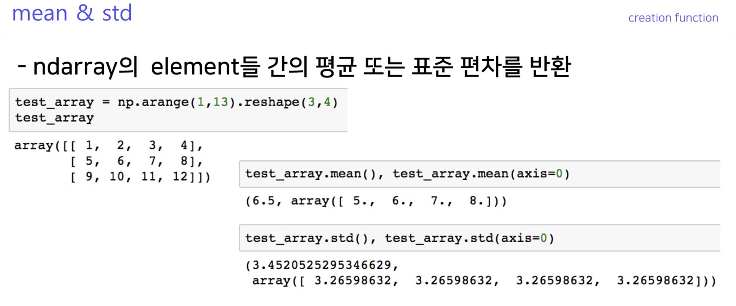
행렬 원소간의 평균과 표준편차를 구함
concat
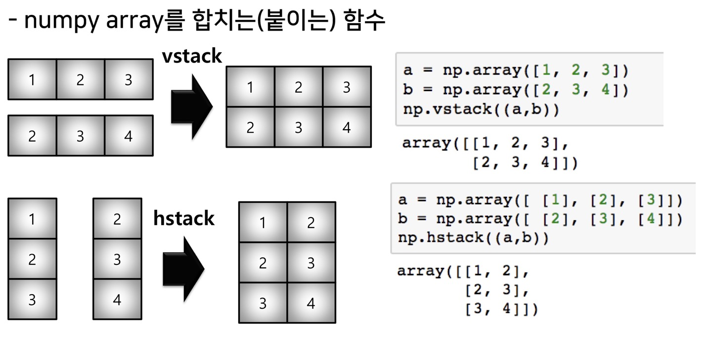
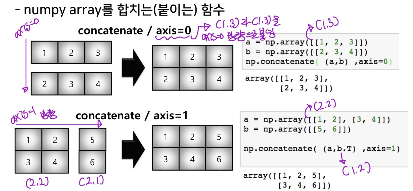
행렬 원소들을 합칠수 있는 함수(b.T는 전치행렬)
array operations
broadcasting
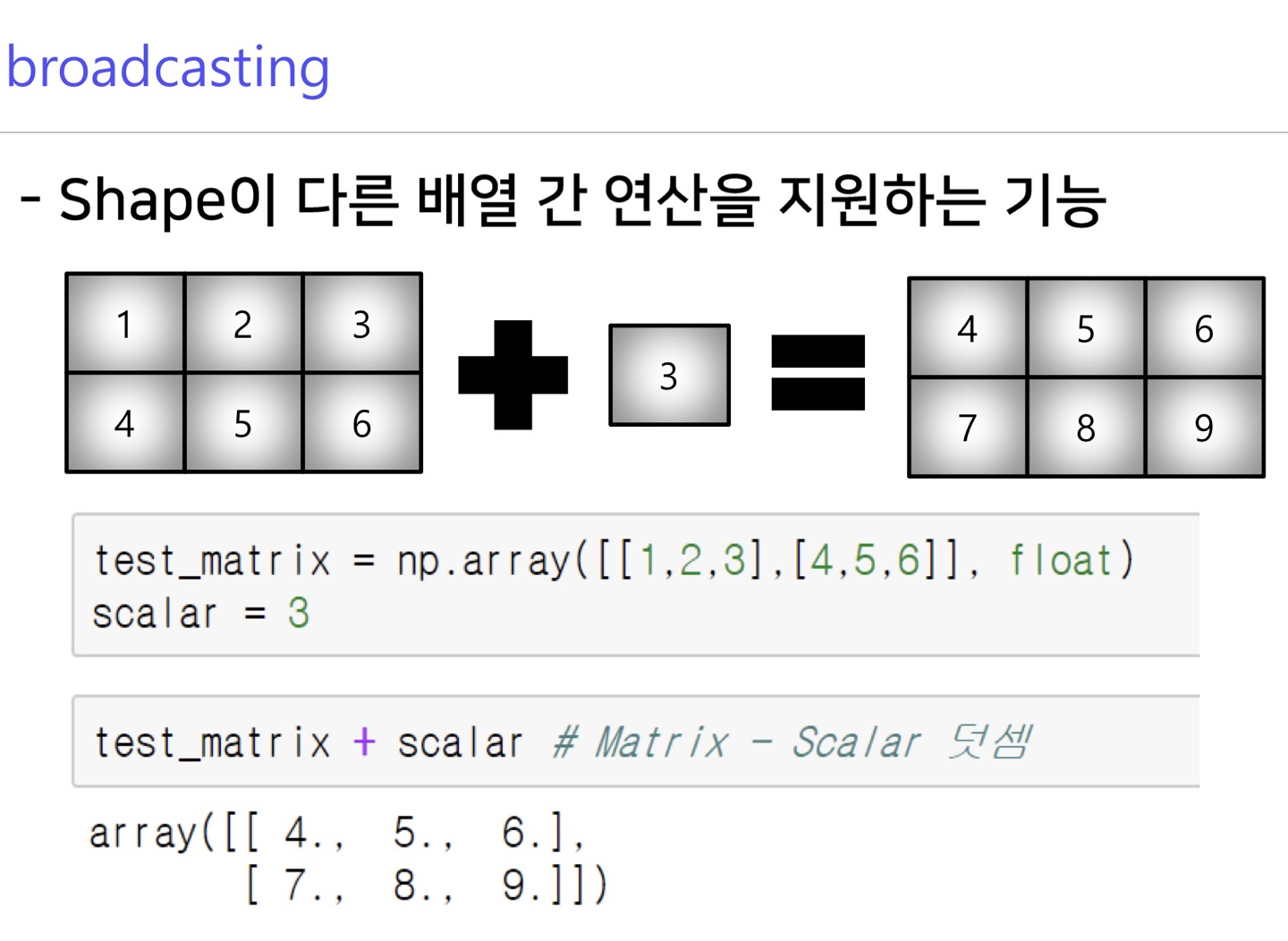
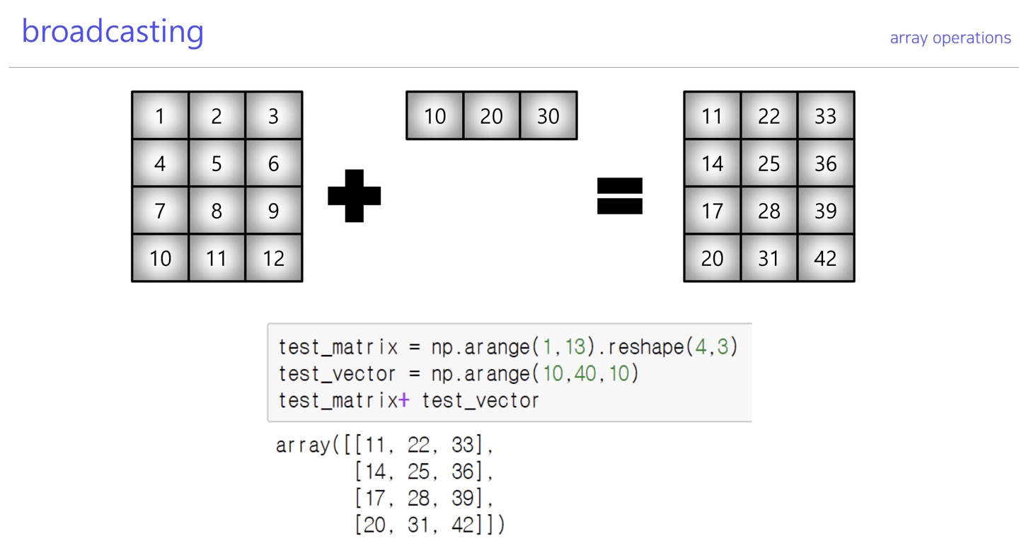
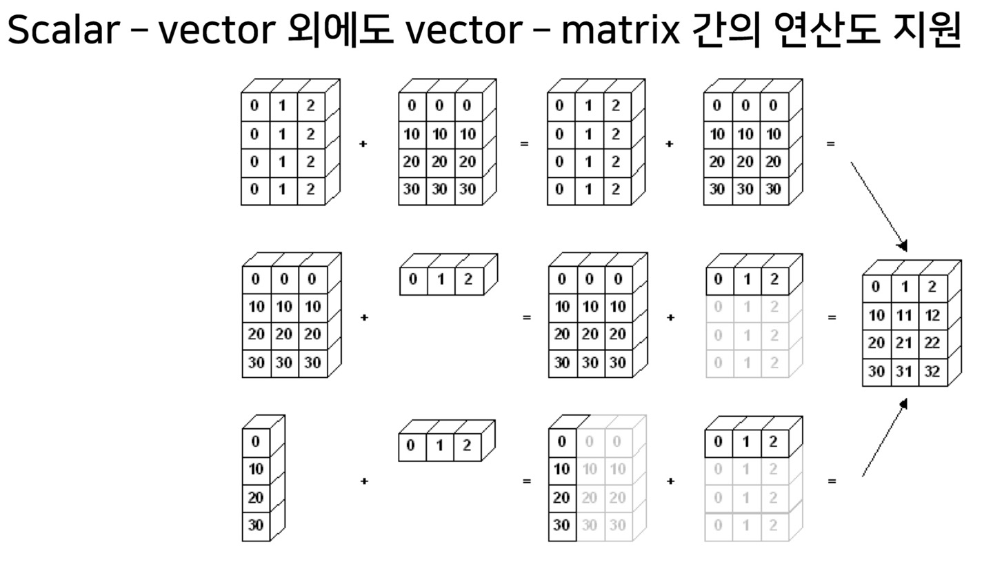
넘파이 rank가 스칼라(0),백터(1)은 나머지 rank들에 대하여 배열간 연산 broadcasting이 가능하다.
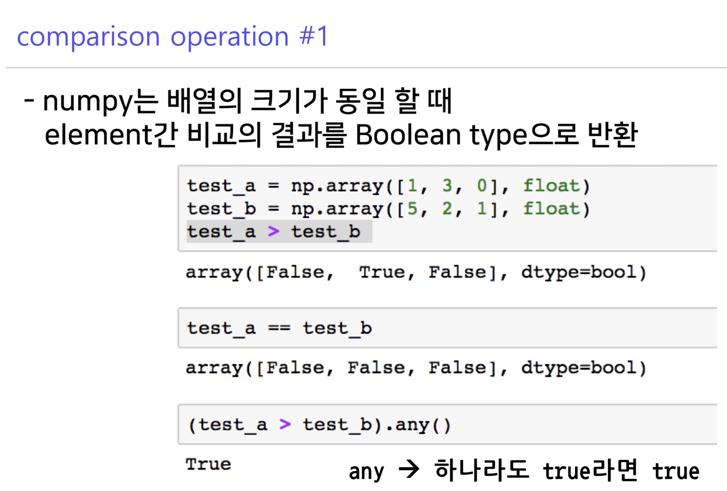
comparisons
all, any
>>> temp=np.arange(10)
>>> temp
array([0, 1, 2, 3, 4, 5, 6, 7, 8, 9])
#any : 원소중 하나라도 조건을 만족하면 true
>>> np.any(temp>5)
True
#all : 모든 원소가 조건을 만족하면 true
>>> np.all(temp<10)
True
>>>
array의 데이터의 일부나 전부가 조건(exp)를 만족하는지 여부를 bool로 리턴
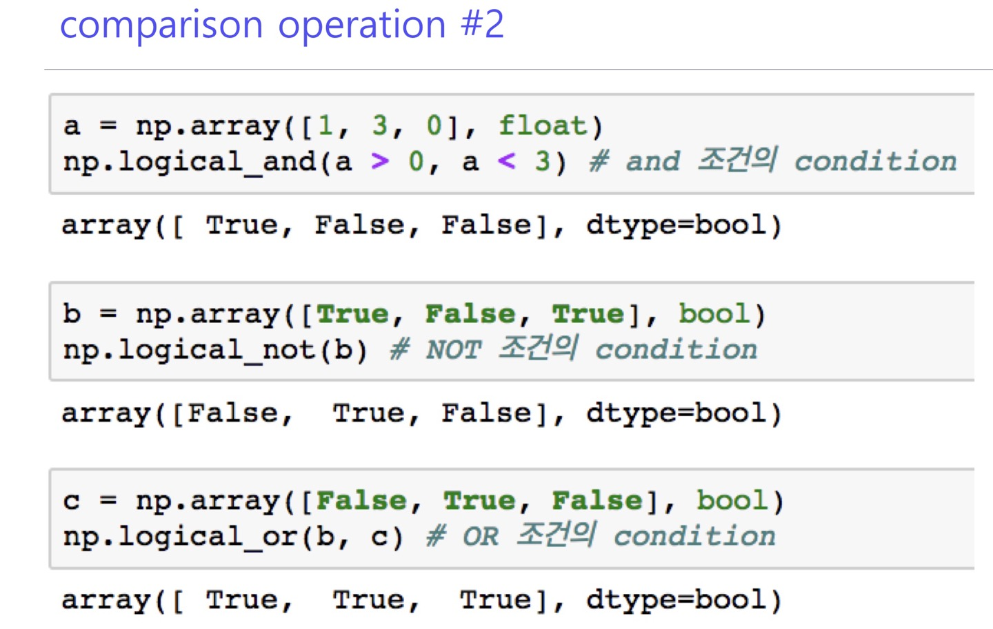
and, or, not
where
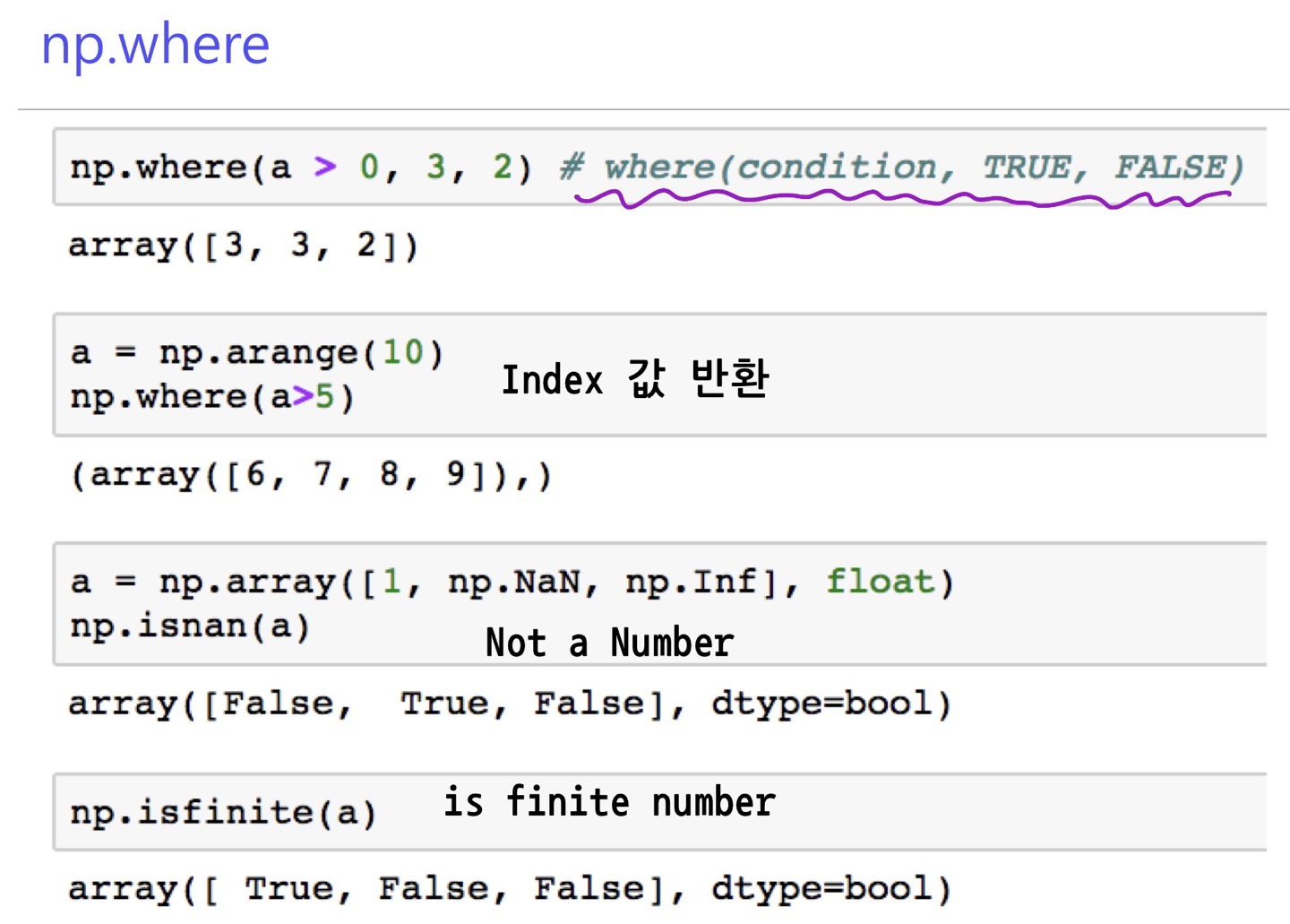
>>> temp=np.arange(10,0,-1)
>>> temp
array([10,  9,  8,  7,  6,  5,  4,  3,  2,  1])
>>> np.where(temp>5)
(array([0, 1, 2, 3, 4], dtype=int64),)
>>>
argmax, argmin
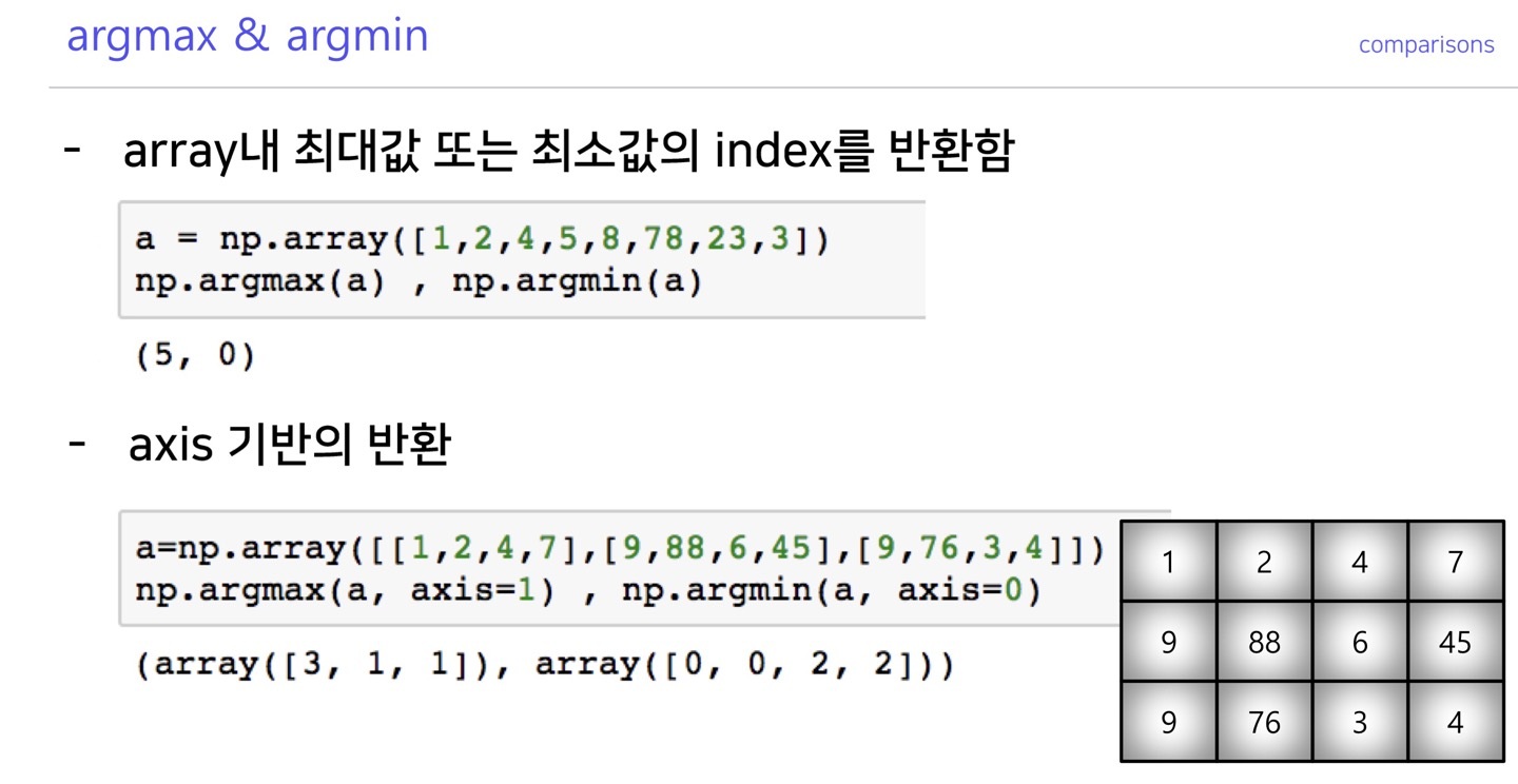
원소중 최대값이나 최소값의 index를 리턴함
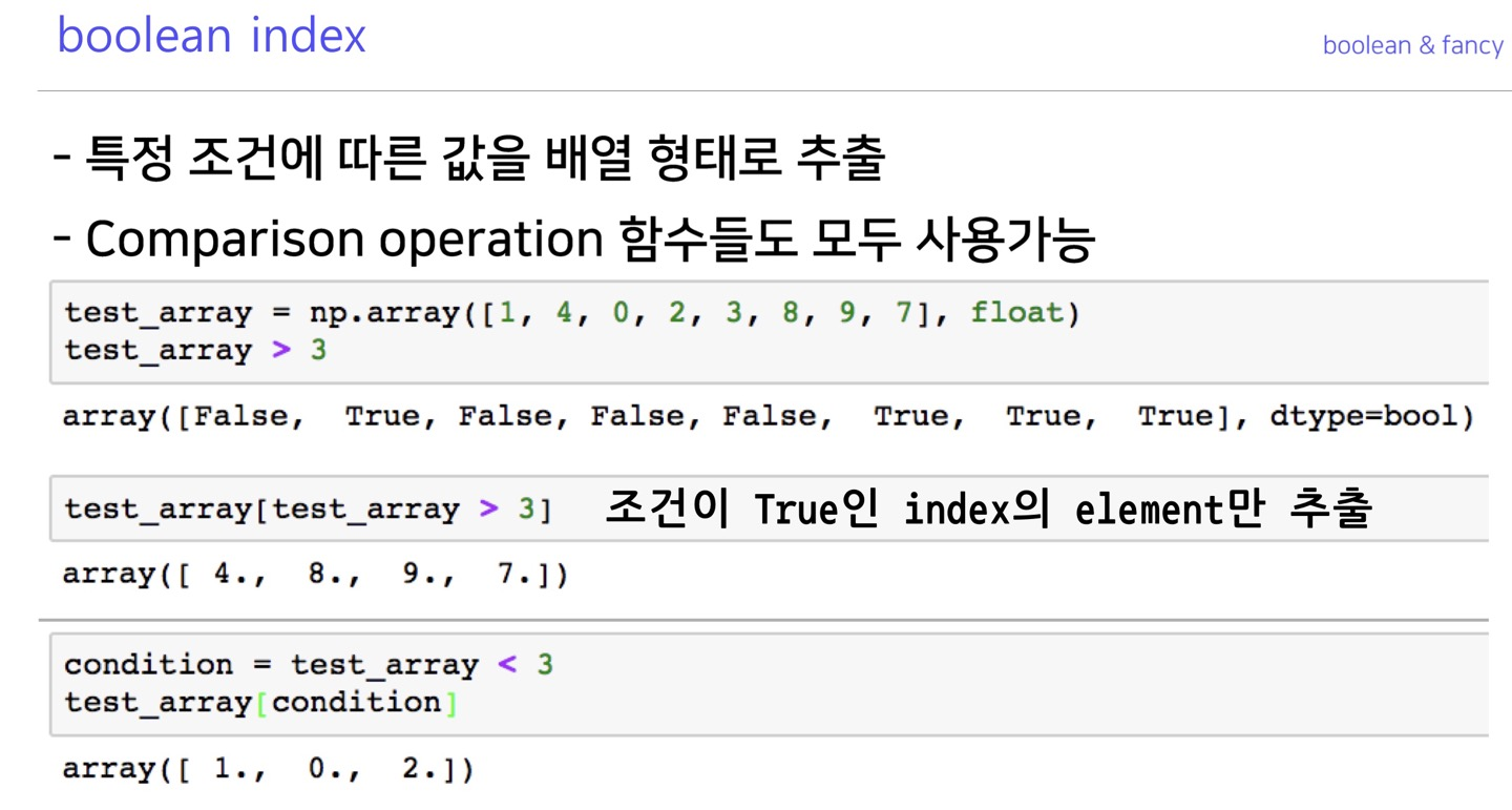
boolean index, fancy index
boolean index
>>> temp
array([[10, 9, 8, 7, 6],
[ 5, 4, 3, 2, 1]])
>>> boolidx=temp>5
>>> boolidx
array([[ True, True, True, True, True],
[False, False, False, False, False]])
>>> temp[boolidx]
array([10, 9, 8, 7, 6])
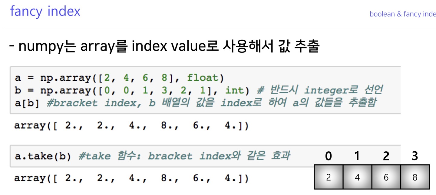
>>>fancy index
numpy io
loadtxt, savetxt
#savetxt
#numpy.savetxt( filename, X, fmt='%.18e', delimiter=' ',
#	newline='n', header='', footer='', comment='#', encoding=None)
#numpy.savetxt({파일이름}, {데이터}, fmt={데이터 형식}, delimiter={데이터간 구분자})
np.savetxt("save.txt", numbers, fmt='%d', delimiter=',')
#loadtxt
#numpy.loadtxt(fname, dtype=<class 'float', comments='#', delimiter=' ',
# conerters=None, skiprows=0, usecols=None, unpack=False, ndmin=0,
# encoding='bytes', max_rows=None>
#numpy.loadtxt({파일 이름}, delimiter=",")
a = np.loadtxt("save.txt", delimiter=",")구분자 지정을 명확하게 해줄것
Pandas I
Pandas init
>>> import pandas as pd
>>> temp=pd.read_csv('sample.csv')
>>> type(temp)
<class 'pandas.core.frame.DataFrame'>
>>> temp.head()
   Emp ID Name Prefix First Name Middle Initial Last Name  ... State    Zip     Region   User Name        Password
0  677509        Drs.       Lois              H    Walker  ...    CO  80224       West    lhwalker   DCa}.T}X:v?NP
1  940761         Ms.     Brenda              S  Robinson  ...    LA  71078      South  bsrobinson   TCo\j#Zg;SQ~o
2  428945         Dr.        Joe              W  Robinson  ...    IN  46057    Midwest  jwrobinson    GO4$J8MiEh[A
3  408351        Drs.      Diane              I     Evans  ...    PA  16328  Northeast     dievans   0gGRtp1HfL<r5
4  193819         Mr.   Benjamin              R   Russell  ...    WI  54940    Midwest   brrussell  Rd<Y8cp!@R;*%F

[5 rows x 37 columns]
>>>
판다스에서 read_csv(path)함수로 데이터를 읽으면 dataframe type로 읽어들인다.
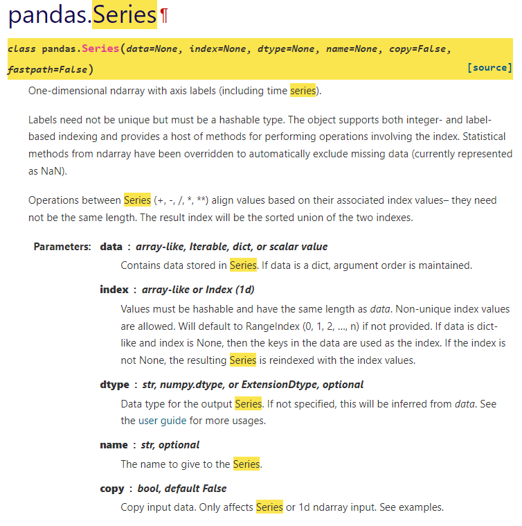
series
#key가 series의 idx로 들어감
>>> dict_data = {'a':1,'b':2,'c':3}
>>> series_data = pd.Series(dict_data)
>>> series_data
a 1
b 2
c 3
dtype: int64
#리스트의 idx가 series의 idx가 됨
>>> list_data = ['2019-01-02',3.14,'ABC',100,True]
>>> series_data2 = pd.Series(list_data)
>>> series_data2
0 2019-01-02
1 3.14
2 ABC
3 100
4 True
dtype: object
#index의 이름을 지정할 수 있다.
>>> idx_name=['a','b','c','d','e']
>>> series_data2 = pd.Series(list_data,index=idx_name)
>>> series_data2
a 2019-01-02
b 3.14
c ABC
d 100
e True
dtype: object
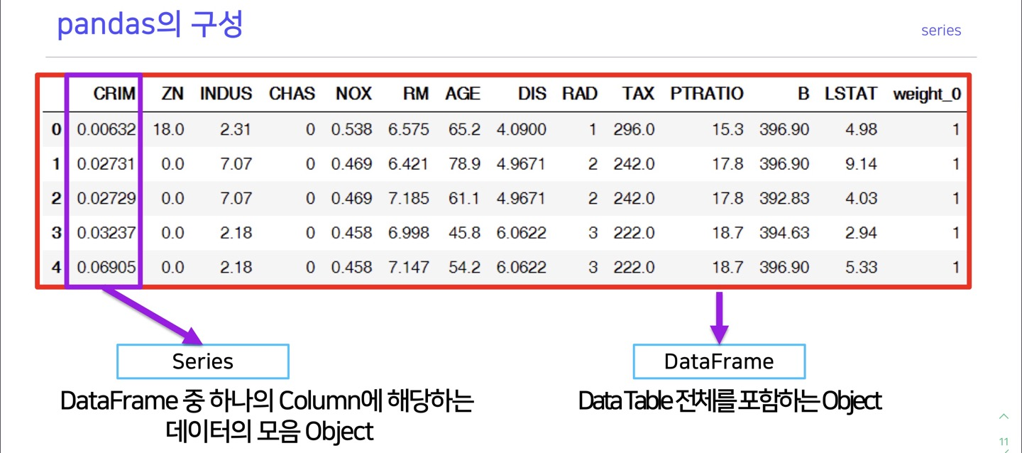
>>>하나의 column에 해당하는 데이터의 모음을 series라고 한다
python 의 dict와 비슷하다고 생각할 수 있다.
dataframe
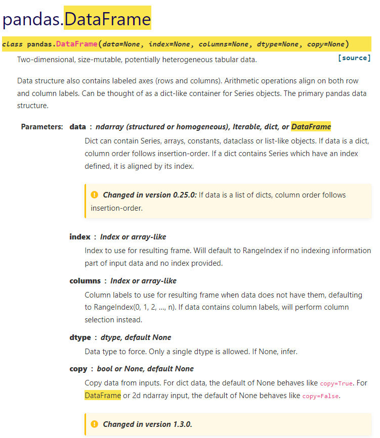
>>> d = {'col1': [1, 2], 'col2': [3, 4]}
>>> df = pd.DataFrame(data=d)
>>> df
   col1  col2
0     1     3
1     2     4
>>>
dataframe indexing
pandas doc : loc
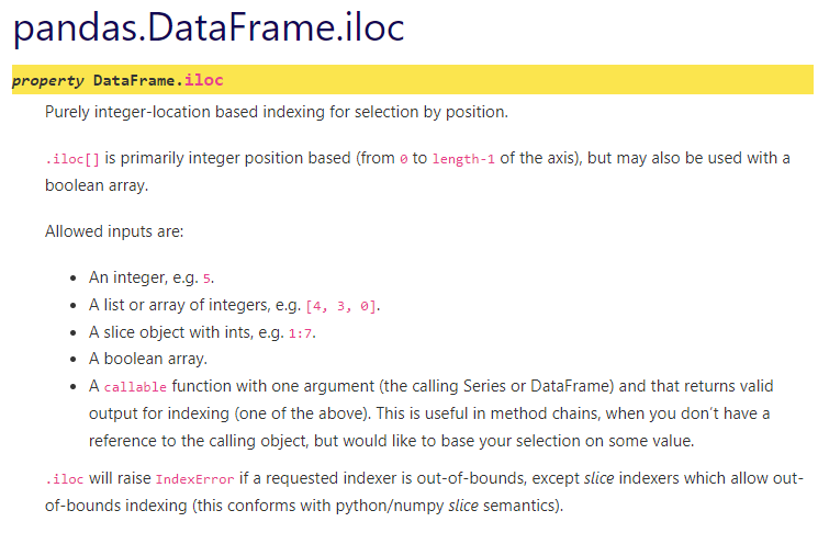
pandas doc : iloc
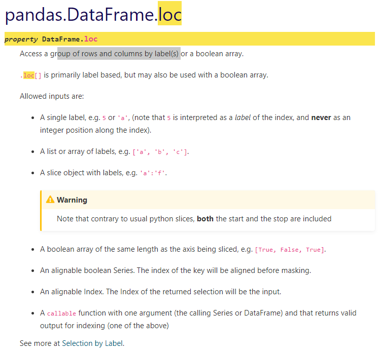
loc : 행이나 열의 라벨을 기준으로 데이터를 그룹지어 줌
iloc : 행이나 열의 idx를 기준으로 데이터를 그룹지어 줌
1개의 열이나 행은 series 2개 이상의 열이나 행은 dataframe type으로 리턴해 준다.
selection & drop
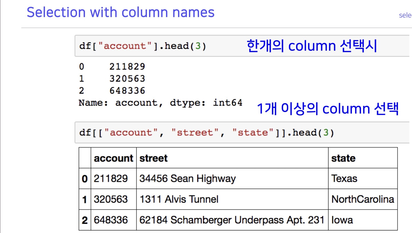
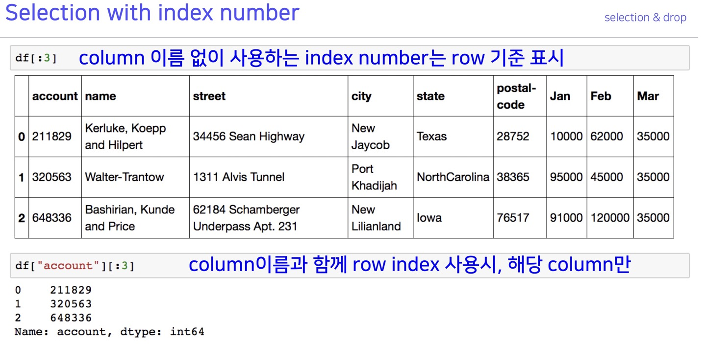
selection
>>> tempcsv=pd.read_csv('sample.csv')
>>> tempcsv.head()
Emp ID Name Prefix First Name Middle Initial Last Name ... State Zip Region User Name Password
0 677509 Drs. Lois H Walker ... CO 80224 West lhwalker DCa}.T}X:v?NP
1 940761 Ms. Brenda S Robinson ... LA 71078 South bsrobinson TCo\j#Zg;SQ~o
2 428945 Dr. Joe W Robinson ... IN 46057 Midwest jwrobinson GO4$J8MiEh[A
3 408351 Drs. Diane I Evans ... PA 16328 Northeast dievans 0gGRtp1HfL<r5
4 193819 Mr. Benjamin R Russell ... WI 54940 Midwest brrussell Rd<Y8cp!@R;*%F
[5 rows x 37 columns]
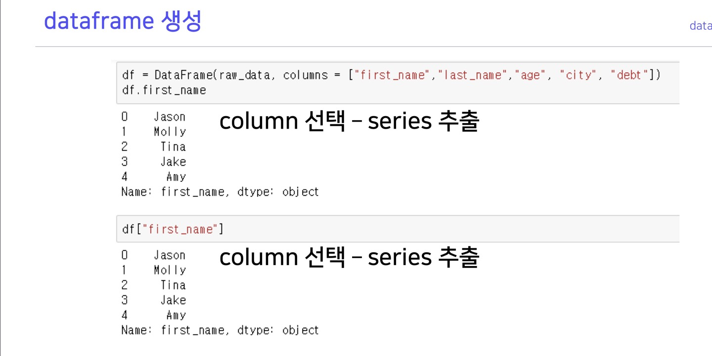
>>> type(tempcsv['Zip'])
<class 'pandas.core.series.Series'>
>>> type(tempcsv[['Zip','Region']])
<class 'pandas.core.frame.DataFrame'>
>>>dataframe['label'], dataframe[[label_list]]
1개의 열이나 행은 series 2개 이상의 열이나 행은 dataframe type으로 리턴해 준다.
data drop
pandas doc : drop
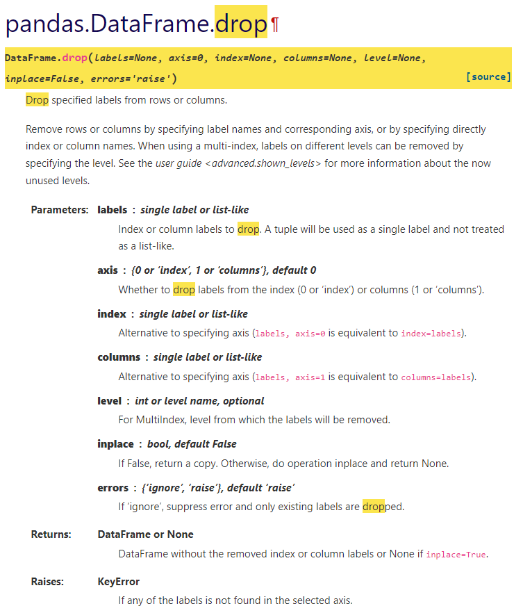
axis의 의미 : n tensor에서 맨 앞부터 0,1,2,3.. 이므로 2x2행렬에서 axis=0은 행이다.
>>> df = pd.DataFrame(np.arange(12).reshape(3, 4),
...                   columns=['A', 'B', 'C', 'D'])
>>> df
   A  B   C   D
0  0  1   2   3
1  4  5   6   7
2  8  9  10  11

#axis=1 : 2x2 에서 axis=1 은 열이므로 b,c 열을 제거
>>> df.drop(['B', 'C'], axis=1)
   A   D
0  0   3
1  4   7
2  8  11

#axis=0 : 2x2 에서 axis=0은 행이므로 0,1 행을 제거
>>> df.drop([0, 1], axis=0)
   A  B   C   D
2  8  9  10  11
>>>
map, apply
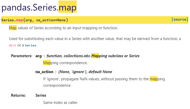
map
>>> s = pd.Series(['cat', 'dog', np.nan, 'rabbit'])
>>> s
0 cat
1 dog
2 NaN
3 rabbit
dtype: object
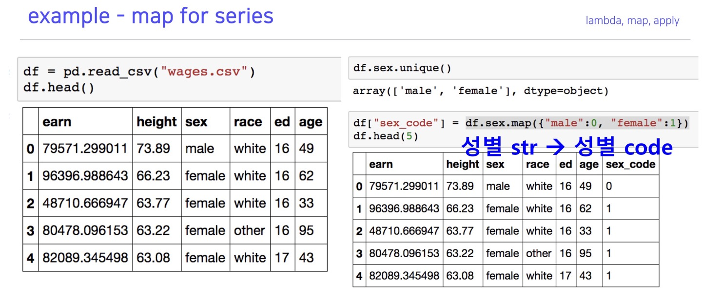
# cat을 kitten으로, dog를 puppy로 맵핑
# data['Sex'] = self.data['Sex'].map({'male':0, 'female':1}) 이런식으로 사용
>>> s.map({'cat': 'kitten', 'dog': 'puppy'})
0 kitten
1 puppy
2 NaN
3 NaN
dtype: object
>>> s.map('I am a {}'.format)
0 I am a cat
1 I am a dog
2 I am a nan
3 I am a rabbit
dtype: object
>>> temp=np.arange(10)
>>> temp=pd.Series(temp)
>>> type(temp)
<class 'pandas.core.series.Series'>
>>> temp
0 0
1 1
2 2
3 3
4 4
5 5
6 6
7 7
8 8
9 9
dtype: int32
#맵함수에 lambda 함수 적용 가능
>>> temp.map(lambda x:x*2)
0 0
1 2
2 4
3 6
4 8
5 10
6 12
7 14
8 16
9 18
dtype: int64
>>>
apply
pandas doc : apply
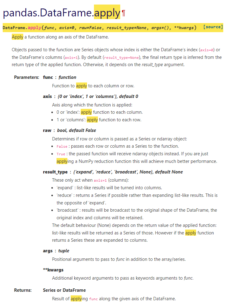
map은 series(단일컬럼)에만 적용이 되고
apply는 dataframe(다중컬럼)에 적용이 된다.
다른 기능은 동일
>>> df = pd.DataFrame(np.arange(12).reshape(3, 4),columns=['A', 'B', 'C', 'D'])
>>> df
   A  B   C   D
0  0  1   2   3
1  4  5   6   7
2  8  9  10  11

#다중컬럼에 map을 적용시키니 에러가 발생
>>> df.map(lambda x: x*2)
Traceback (most recent call last):
AttributeError: 'DataFrame' object has no attribute 'map'

#apply는 에러가 발생하지 않음
>>> df.apply(lambda x: x*2)
    A   B   C   D
0   0   2   4   6
1   8  10  12  14
2  16  18  20  22
>>>
pandas built-in functions
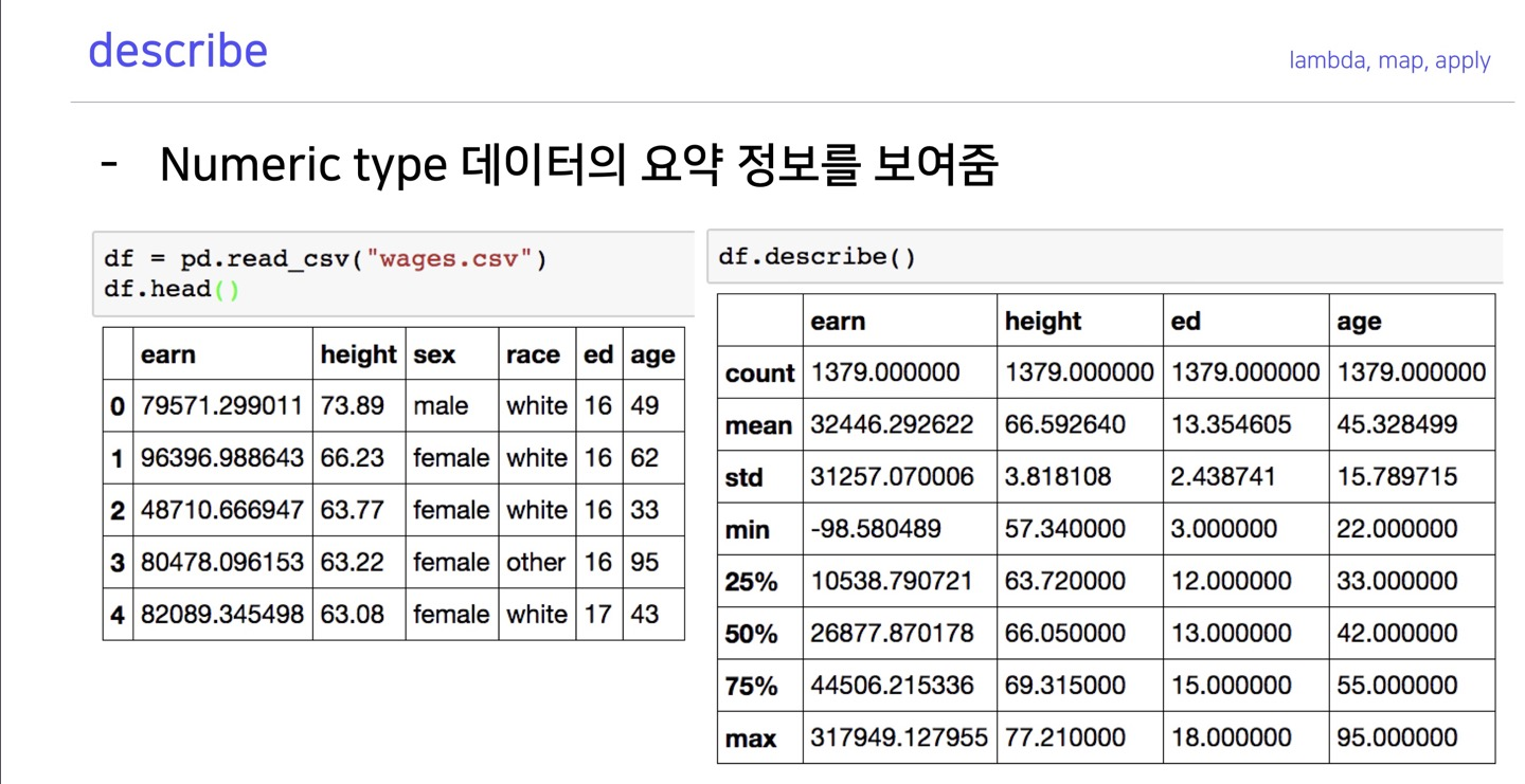
describe
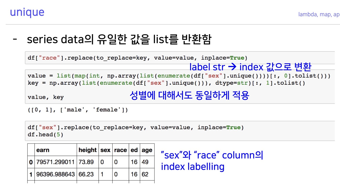
unique
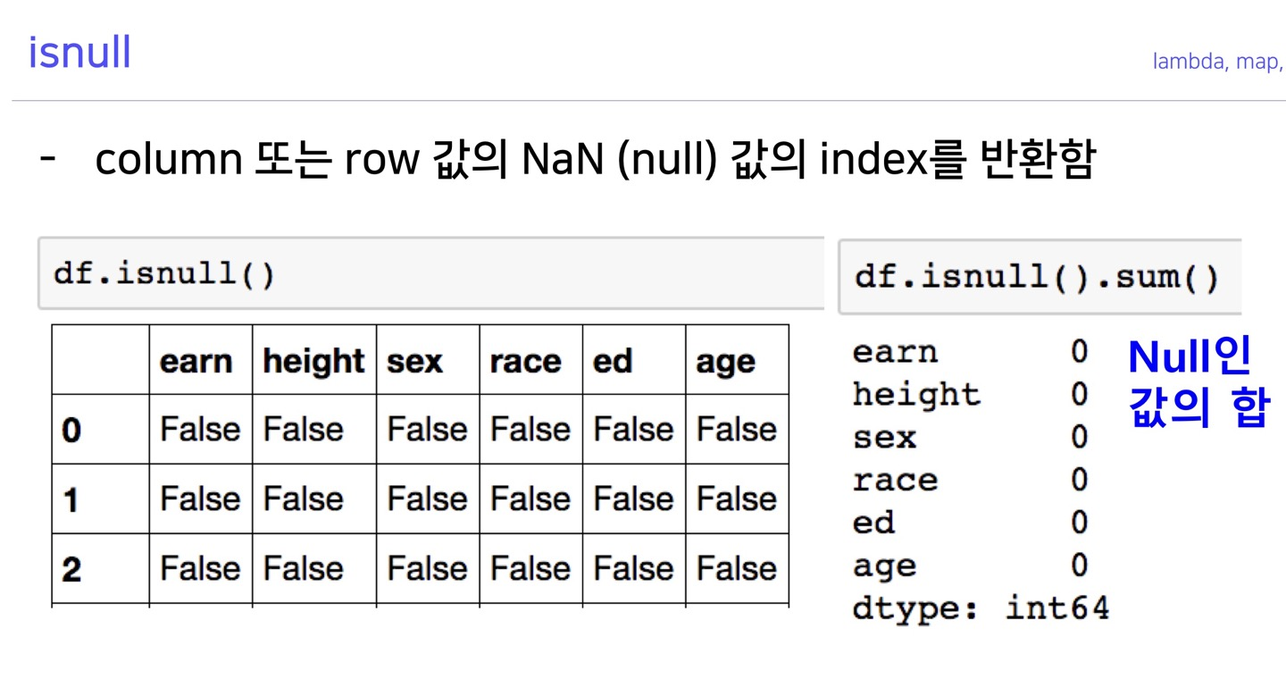
isnull
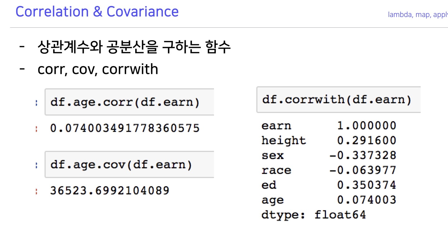
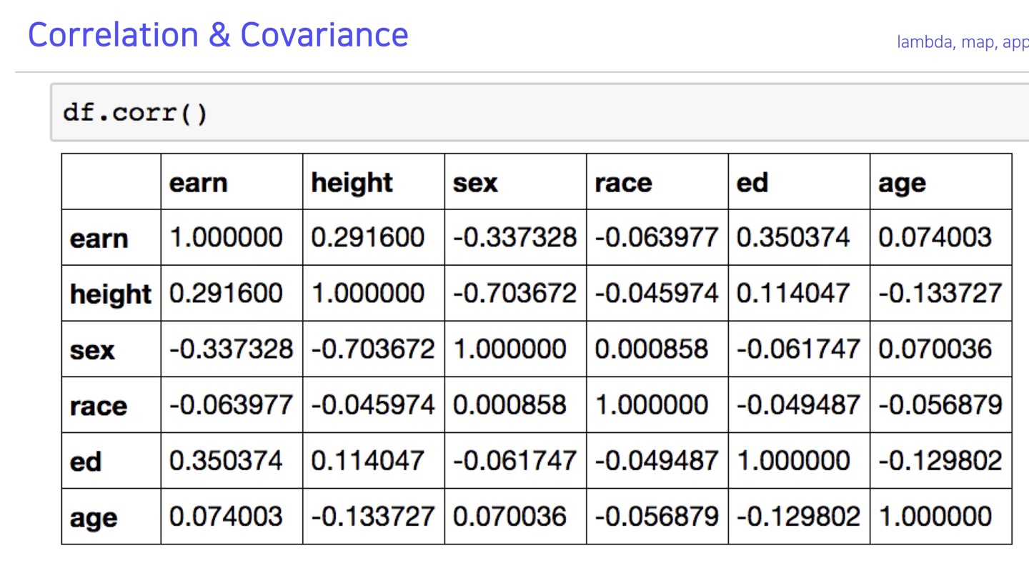
correlation & covariance
pandas doc : corr
pandas doc : cov
pandas doc : corrwith
Pandas II
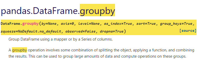
Groupby I
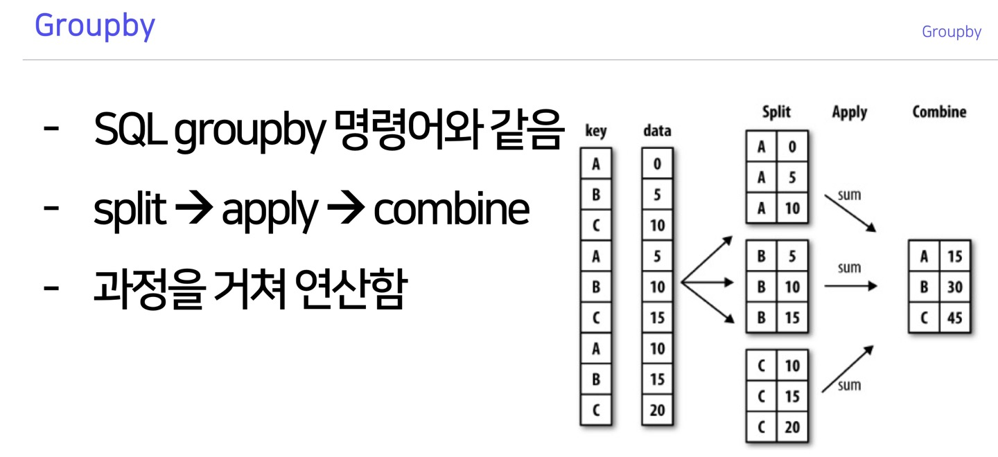
Groupby
>>> df = pd.DataFrame({'Animal': ['Falcon', 'Falcon',
...                               'Parrot', 'Parrot'],
...                    'Max Speed': [380., 370., 24., 26.]})
>>> df
   Animal  Max Speed
0  Falcon      380.0
1  Falcon      370.0
2  Parrot       24.0
3  Parrot       26.0
>>> dfg=df.groupby('Animal')
>>> dfg
<pandas.core.groupby.generic.DataFrameGroupBy object at 0x00000188EB23ADC0>

#그룹화된 내용을 보고싶을 경우 apply(print)로 확인가능
>>> dfg.apply(print)
   Animal  Max Speed
0  Falcon      380.0
1  Falcon      370.0
   Animal  Max Speed
2  Parrot       24.0
3  Parrot       26.0
Empty DataFrame
Columns: []
Index: []

#그룹화시킨다음 그룹끼리 행할 연산을 설정가능
>>> dfg.sum()
        Max Speed
Animal
Falcon      750.0
Parrot       50.0
>>>
Hierarchical index
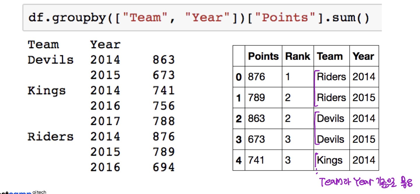
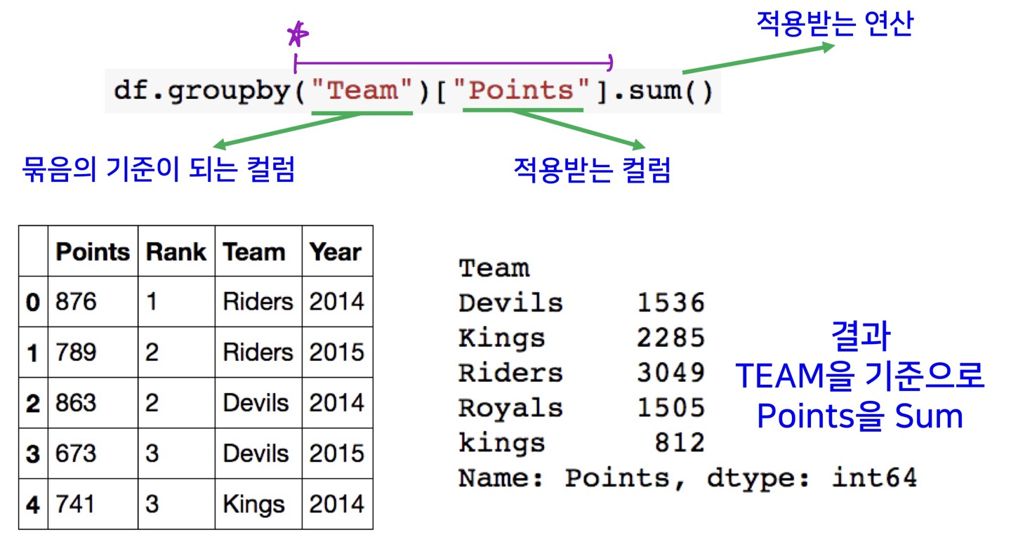
df.groupby([group_list])[target].oper()묶음의 기준이 되는 컬럼은 1개 이상이 될 수 있다.
컬럼이 2개 이상이 되면 그룹화 된 이후의 인덱스 역시 2개 이상이 된다.(=Hierarchical index)
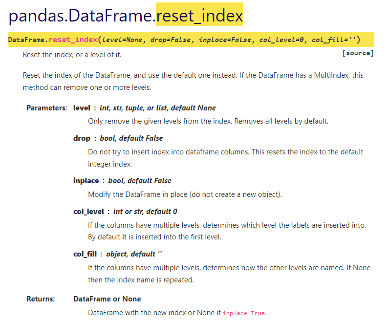
#멀티인덱스를 다시 풀어줄수도 있다.
>>> index = pd.MultiIndex.from_tuples([('bird', 'falcon'),
...                                    ('bird', 'parrot'),
...                                    ('mammal', 'lion'),
...                                    ('mammal', 'monkey')],
...                                   names=['class', 'name'])
>>> columns = pd.MultiIndex.from_tuples([('speed', 'max'),
...                                      ('species', 'type')])
>>> df = pd.DataFrame([(389.0, 'fly'),
...                    ( 24.0, 'fly'),
...                    ( 80.5, 'run'),
...                    (np.nan, 'jump')],
...                   index=index,
...                   columns=columns)
>>> df
               speed species
                 max    type
class  name
bird   falcon  389.0     fly
       parrot   24.0     fly
mammal lion     80.5     run
       monkey    NaN    jump
>>> df.reset_index()
    class    name  speed species
                     max    type
0    bird  falcon  389.0     fly
1    bird  parrot   24.0     fly
2  mammal    lion   80.5     run
3  mammal  monkey    NaN    jump
Hierarchical index-unstack
pandas doc : unstack
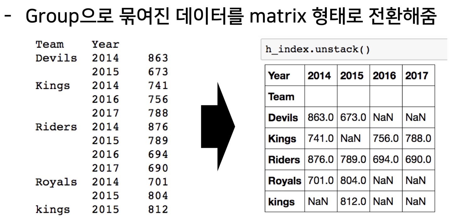
그룹으로 묶여서 연산된 데이터를 matrix 형식으로 전환해줌
>>> index = pd.MultiIndex.from_tuples([('one', 'a'), ('one', 'b'),
...                                    ('two', 'a'), ('two', 'b')])
>>> s = pd.Series(np.arange(1.0, 5.0), index=index)
>>> s
one  a    1.0
     b    2.0
two  a    3.0
     b    4.0
dtype: float64
>>> s.unstack()
       a    b
one  1.0  2.0
two  3.0  4.0
>>>
Hierarchical index-swaplevel
>>> index = pd.MultiIndex.from_tuples([('bird', 'falcon'),
... ('bird', 'parrot'),
... ('mammal', 'lion'),
... ('mammal', 'monkey')],
... names=['class', 'name'])
>>> columns = pd.MultiIndex.from_tuples([('speed', 'max'),
... ('species', 'type')])
>>> df = pd.DataFrame([(389.0, 'fly'),
... ( 24.0, 'fly'),
... ( 80.5, 'run'),
... (np.nan, 'jump')],
... index=index,
... columns=columns)
>>> df
speed species
max type
class name
bird falcon 389.0 fly
parrot 24.0 fly
mammal lion 80.5 run
monkey NaN jump
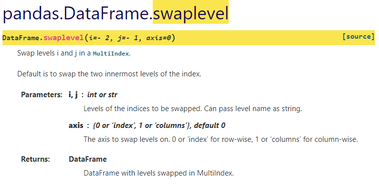
#index의 레벨이 서로 바뀌었음 (class<->name)
>>> df.swaplevel()
speed species
max type
name class
falcon bird 389.0 fly
parrot bird 24.0 fly
lion mammal 80.5 run
monkey mammal NaN jump
>>>Hierarchical index-sortlevel
pandas doc : sortlevel
pandas doc : sort_values
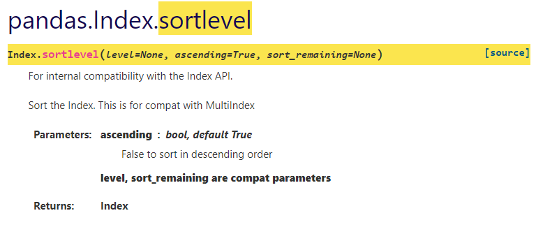
인덱스 기준으로 정렬을 할 수 있음.
(value를 기준으로 정렬할려면 sort_values)
Groupby II
Grouped
for 문을 사용해 grouped 된 상태를 튜플 형태로 추출할 수 있다.
>>> df = pd.DataFrame({'Animal': ['Falcon', 'Falcon',
...                               'Parrot', 'Parrot'],
...                    'Max Speed': [380., 370., 24., 26.]})
>>> df
   Animal  Max Speed
0  Falcon      380.0
1  Falcon      370.0
2  Parrot       24.0
3  Parrot       26.0
>>> gdf=df.groupby(['Animal'])
>>> for name,group in gdf:
...     print(name)
...     print(group)
...
Falcon
   Animal  Max Speed
0  Falcon      380.0
1  Falcon      370.0
Parrot
   Animal  Max Speed
2  Parrot       24.0
3  Parrot       26.0

#특정 key 값을 가진 그룹만 추출이 가능하다.
>>> gdf.get_group('Falcon')
   Animal  Max Speed
0  Falcon      380.0
1  Falcon      370.0
>>>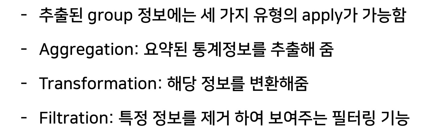
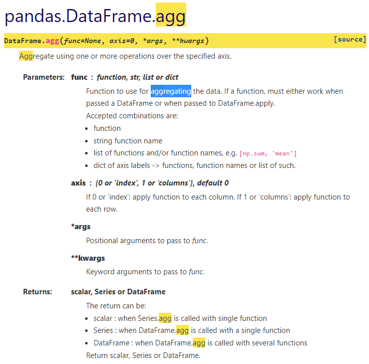
aggregation (합계)
>>> gdf.agg(sum)
        Max Speed
Animal
Falcon      750.0
Parrot       50.0
>>> import numpy as np
>>> gdf.agg(np.mean)
        Max Speed
Animal
Falcon      375.0
Parrot       25.0

#여러 연산을 한번에 적용할 수 있음
>>> gdf.agg([np.mean,sum,np.std])
       Max Speed
            mean    sum       std
Animal
Falcon     375.0  750.0  7.071068
Parrot      25.0   50.0  1.414214
>>>
그룹화된(grouped) 자료에 agg 연산을
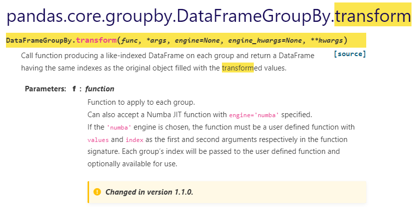
transformation
>>> df = pd.DataFrame({'A' : ['foo', 'bar', 'foo', 'bar',
...                           'foo', 'bar'],
...                    'B' : ['one', 'one', 'two', 'three',
...                           'two', 'two'],
...                    'C' : [1, 5, 5, 2, 5, 5],
...                    'D' : [2.0, 5., 8., 1., 2., 9.]})
>>> grouped = df.groupby('A')
>>> df
     A      B  C    D
0  foo    one  1  2.0
1  bar    one  5  5.0
2  foo    two  5  8.0
3  bar  three  2  1.0
4  foo    two  5  2.0
5  bar    two  5  9.0
>>> grouped.apply(print)
     A      B  C    D
1  bar    one  5  5.0
3  bar  three  2  1.0
5  bar    two  5  9.0
     A    B  C    D
0  foo  one  1  2.0
2  foo  two  5  8.0
4  foo  two  5  2.0
Empty DataFrame
Columns: []
Index: []

>>> grouped.transform(lambda x:x*2)
            B   C     D
0      oneone   2   4.0
1      oneone  10  10.0
2      twotwo  10  16.0
3  threethree   4   2.0
4      twotwo  10   4.0
5      twotwo  10  18.0

#결과는 어차피 df 기준으로 나오는듯 하다.
#이럴거면 굳이 grouped에 transform을 적용시키는 이유가 필요없을거같은데..
>>> df.transform(lambda x:x*2)
        A           B   C     D
0  foofoo      oneone   2   4.0
1  barbar      oneone  10  10.0
2  foofoo      twotwo  10  16.0
3  barbar  threethree   4   2.0
4  foofoo      twotwo  10   4.0
5  barbar      twotwo  10  18.0
>>>
>>>
filter (검색)
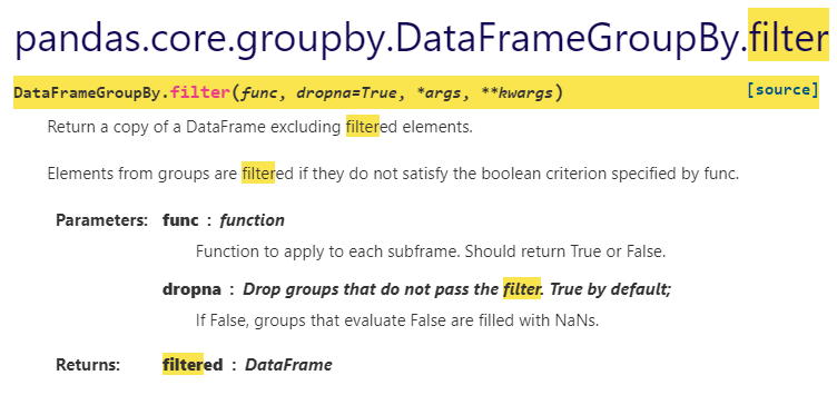
>>> df = pd.DataFrame({'A' : ['foo', 'bar', 'foo', 'bar',
...                           'foo', 'bar'],
...                    'B' : [1, 2, 3, 4, 5, 6],
...                    'C' : [2.0, 5., 8., 1., 2., 9.]})
>>> grouped = df.groupby('A')
>>> grouped.apply(print)
     A  B    C
1  bar  2  5.0
3  bar  4  1.0
5  bar  6  9.0
     A  B    C
0  foo  1  2.0
2  foo  3  8.0
4  foo  5  2.0
Empty DataFrame
Columns: []
Index: []
>>> grouped.filter(lambda x: x['B'].mean() > 3.)
     A  B    C
1  bar  2  5.0
3  bar  4  1.0
5  bar  6  9.0

# 그룹화된 df 객체의 컬럼의 합의 평균...
>>> grouped.agg(np.mean)
     B    C
A
bar  4  5.0
foo  3  4.0
>>>

# 바로 df에 filter를 적용하면 적용되지 않음(where 사용하면됨)
>>> df.filter(lambda x: x['B'].mean() > 3.)
Traceback (most recent call last):
  File "<stdin>", line 1, in <module>
  File "C:\Users\AI01\anaconda3\lib\site-packages\pandas\core\generic.py", line 4976, in filter
    return self.reindex(**{name: [r for r in items if r in labels]})
TypeError: 'function' object is not iterable
>>>
Pivot table Crosstab
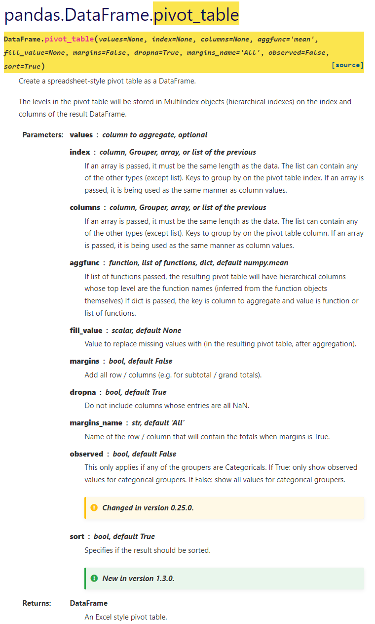
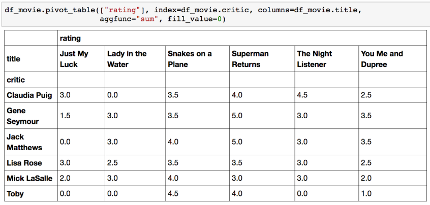
Pivot table
피벗 테이블(pivot table)은 커다란 표(예: 데이터베이스, 스프레드시트, 비즈니스 인텔리전스 프로그램 등)의 데이터를 요약하는 통계표이다. 이 요약에는 합계, 평균, 기타 통계가 포함될 수 있으며 피벗 테이블이 이들을 함께 의미있는 방식으로 묶어준다.
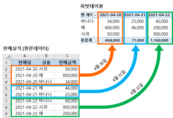
우리가 excel에서 보던 그 것!
Index 축은 groupby와 동일함
Column에 추가로 labeling 값을 추가하여,
Value에 numeric type 값을 aggregation 하는 형태
>>> df = pd.DataFrame({"A": ["foo", "foo", "foo", "foo", "foo",
... "bar", "bar", "bar", "bar"],
... "B": ["one", "one", "one", "two", "two",
... "one", "one", "two", "two"],
... "C": ["small", "large", "large", "small",
... "small", "large", "small", "small",
... "large"],
... "D": [1, 2, 2, 3, 3, 4, 5, 6, 7],
... "E": [2, 4, 5, 5, 6, 6, 8, 9, 9]})
>>> df
A B C D E
0 foo one small 1 2
1 foo one large 2 4
2 foo one large 2 5
3 foo two small 3 5
4 foo two small 3 6
5 bar one large 4 6
6 bar one small 5 8
7 bar two small 6 9
8 bar two large 7 9
# agg 연산(np.sum)이 적용될 값을 D 로 하고, 인덱스는 A,B의 그룹(foo,one)을 인덱스로 사용한다.
# 그리고 열은 C의 원소들(small, large)을 사용한다.
>>> df.pivot_table(values=['D'],index=['A','B'],columns=['C'],aggfunc=np.sum)
D
C large small
A B
bar one 4.0 5.0
two 7.0 6.0
foo one 4.0 1.0
two NaN 6.0
>>> table = pd.pivot_table(df, values='D', index=['A', 'B'],
... columns=['C'], aggfunc=np.sum)
>>> table
C large small
A B
bar one 4.0 5.0
two 7.0 6.0
foo one 4.0 1.0
two NaN 6.0
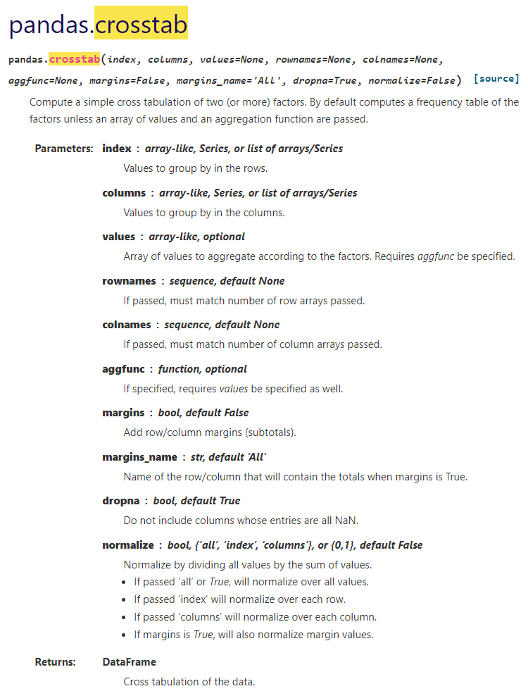
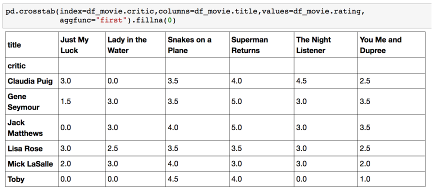
>>>Crosstab
두 칼럼에 교차 빈도, 비율, 덧셈 등을 구할 때 사용
Pivot table의 특수한 형태
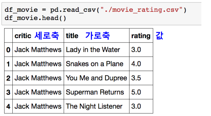
User-Item Rating Matrix 등을 만들 때 사용가능함
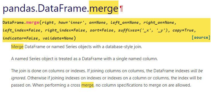
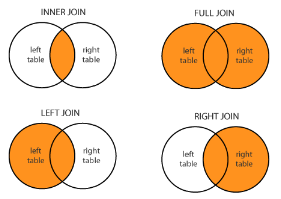
Merge & Concat
Merge
두개의 df를 columns을 기준으로 합침
>>> df1 = pd.DataFrame({'lkey': ['foo', 'bar', 'baz', 'foo'],
...                     'value': [1, 2, 3, 5]})
>>> df2 = pd.DataFrame({'rkey': ['foo', 'bar', 'baz', 'foo'],
...                     'value': [5, 6, 7, 8]})
>>> df1
  lkey  value
0  foo      1
1  bar      2
2  baz      3
3  foo      5
>>> df2
  rkey  value
0  foo      5
1  bar      6
2  baz      7
3  foo      8
>>> df1.merge(df2, left_on='lkey', right_on='rkey')
  lkey  value_x rkey  value_y
0  foo        1  foo        5
1  foo        1  foo        8
2  foo        5  foo        5
3  foo        5  foo        8
4  bar        2  bar        6
5  baz        3  baz        7
>>>
>>> df1 = pd.DataFrame({'a': ['foo', 'bar'], 'b': [1, 2]})
>>> df2 = pd.DataFrame({'a': ['foo', 'baz'], 'c': [3, 4]})
>>> df1
a b
0 foo 1
1 bar 2
>>> df2
a c
0 foo 3
1 baz 4
# df1 과 df2 a에 대해서 inner join -> foo 밖에 없음
>>> df1.merge(df2, how='inner', on='a')
a b c
0 foo 1 3
# a 에 대해서 left join -> df1이 left이므로 -> foo, bar(bar는 우측 테이블에 없으므로 nan)
>>> df1.merge(df2, how='left', on='a')
a b c
0 foo 1 3.0
1 bar 2 NaN
>>> pd.merge(df1,df2, how='left', on='a')
a b c
0 foo 1 3.0
1 bar 2 NaN
>>> pd.merge(df1,df2, how='outer', on='a')
a b c
0 foo 1.0 3.0
1 bar 2.0 NaN
2 baz NaN 4.0
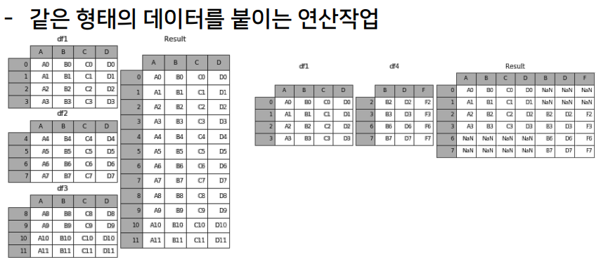
>>>Concat
>>> df1 = pd.DataFrame([['a', 1], ['b', 2]],
... columns=['letter', 'number'])
>>> df1
letter number
0 a 1
1 b 2
>>> df2 = pd.DataFrame([['c', 3], ['d', 4]],
... columns=['letter', 'number'])
>>> df2
letter number
0 c 3
1 d 4
>>> pd.concat([df1, df2])
letter number
0 a 1
1 b 2
0 c 3
1 d 4
>>>
>>> pd.concat([df1, df2]).reset_index()
index letter number
0 0 a 1
1 1 b 2
2 0 c 3
3 1 d 4
>>> pd.concat([df1, df2]).reset_index(drop=True)
letter number
0 a 1
1 b 2
2 c 3
3 d 4
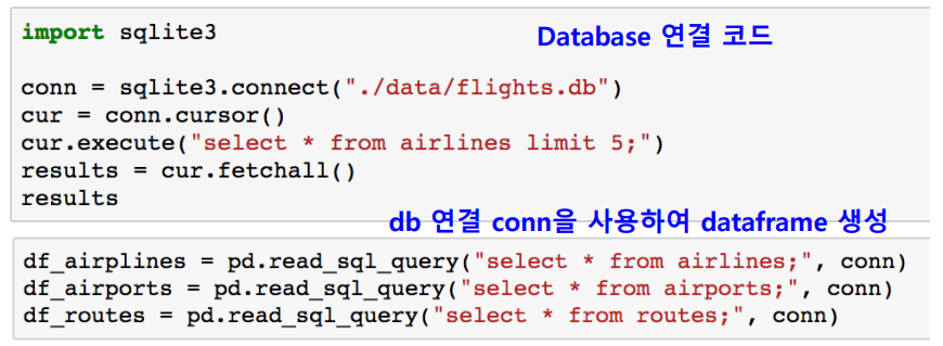
>>>persistence
Database connection
Data loading시 db connection 기능을 제공함
XLS persistence
Dataframe의 엑셀 추출 코드
Xls 엔진으로 openpyxls 또는 XlsxWrite 사용

Pickle persistence
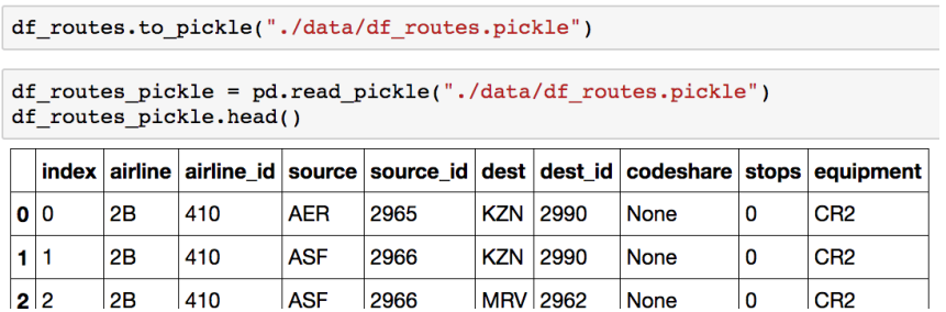
가장 일반적인 python 파일 persistence
to_pickle, read_pickle 함수 사용