Body signal of smoking
데이터 출처
This dataset is a collection of basic health biological signal data.
The goal is to determine the presence or absence of smoking through bio-signals.
데이터는 총 27개의 칼럼과 55692개의 rows로 구성
| Header | Description |
|---|---|
| ID | index |
| gender | - |
| age | 5-years gap |
| height(cm) | - |
| weight(kg) | - |
| waist(cm) | waist circumference length |
| eyesight(left) | - |
| eyesight(right) | - |
| hearing(left) | - |
| hearing(right) | - |
| systolic | Blood pressure |
| relaxation | Blood pressure |
| fasting blood sugar | - |
| Cholesterol | total |
| triglyceride | - |
| HDL | cholesterol type |
| LDL | cholesterol type |
| hemoglobin | - |
| Urine protein | - |
| serum creatinine | - |
| AST | glutamic oxaloacetic transaminase type |
| ALT | glutamic oxaloacetic transaminase type |
| Gtp | γ-GTP |
| oral | Oral Examination status |
| dental caries | - |
| tartar | tartar status |
| smoking | - |
EDA
- 데이터 구조 파악
df <- read.csv(file = 'smoking.csv', stringsAsFactors = TRUE)
head(df)
##   ID gender age height.cm. weight.kg. waist.cm. eyesight.left. eyesight.right.
## 1  0      F  40        155         60      81.3            1.2             1.0
## 2  1      F  40        160         60      81.0            0.8             0.6
## 3  2      M  55        170         60      80.0            0.8             0.8
## 4  3      M  40        165         70      88.0            1.5             1.5
## 5  4      F  40        155         60      86.0            1.0             1.0
## 6  5      M  30        180         75      85.0            1.2             1.2
##   hearing.left. hearing.right. systolic relaxation fasting.blood.sugar
## 1             1              1      114         73                  94
## 2             1              1      119         70                 130
## 3             1              1      138         86                  89
## 4             1              1      100         60                  96
## 5             1              1      120         74                  80
## 6             1              1      128         76                  95
##   Cholesterol triglyceride HDL LDL hemoglobin Urine.protein serum.creatinine
## 1         215           82  73 126       12.9             1              0.7
## 2         192          115  42 127       12.7             1              0.6
## 3         242          182  55 151       15.8             1              1.0
## 4         322          254  45 226       14.7             1              1.0
## 5         184           74  62 107       12.5             1              0.6
## 6         217          199  48 129       16.2             1              1.2
##   AST ALT Gtp oral dental.caries tartar smoking
## 1  18  19  27    Y             0      Y       0
## 2  22  19  18    Y             0      Y       0
## 3  21  16  22    Y             0      N       1
## 4  19  26  18    Y             0      Y       0
## 5  16  14  22    Y             0      N       0
## 6  18  27  33    Y             0      Y       0
str(df)
## 'data.frame':    55692 obs. of  27 variables:
##  $ ID                 : int  0 1 2 3 4 5 6 7 9 10 ...
##  $ gender             : Factor w/ 2 levels "F","M": 1 1 2 2 1 2 2 2 1 2 ...
##  $ age                : int  40 40 55 40 40 30 40 45 50 45 ...
##  $ height.cm.         : int  155 160 170 165 155 180 160 165 150 175 ...
##  $ weight.kg.         : int  60 60 60 70 60 75 60 90 60 75 ...
##  $ waist.cm.          : num  81.3 81 80 88 86 85 85.5 96 85 89 ...
##  $ eyesight.left.     : num  1.2 0.8 0.8 1.5 1 1.2 1 1.2 0.7 1 ...
##  $ eyesight.right.    : num  1 0.6 0.8 1.5 1 1.2 1 1 0.8 1 ...
##  $ hearing.left.      : num  1 1 1 1 1 1 1 1 1 1 ...
##  $ hearing.right.     : num  1 1 1 1 1 1 1 1 1 1 ...
##  $ systolic           : num  114 119 138 100 120 128 116 153 115 113 ...
##  $ relaxation         : num  73 70 86 60 74 76 82 96 74 64 ...
##  $ fasting.blood.sugar: num  94 130 89 96 80 95 94 158 86 94 ...
##  $ Cholesterol        : num  215 192 242 322 184 217 226 222 210 198 ...
##  $ triglyceride       : num  82 115 182 254 74 199 68 269 66 147 ...
##  $ HDL                : num  73 42 55 45 62 48 55 34 48 43 ...
##  $ LDL                : num  126 127 151 226 107 129 157 134 149 126 ...
##  $ hemoglobin         : num  12.9 12.7 15.8 14.7 12.5 16.2 17 15 13.7 16 ...
##  $ Urine.protein      : num  1 1 1 1 1 1 1 1 1 1 ...
##  $ serum.creatinine   : num  0.7 0.6 1 1 0.6 1.2 0.7 1.3 0.8 0.8 ...
##  $ AST                : num  18 22 21 19 16 18 21 38 31 26 ...
##  $ ALT                : num  19 19 16 26 14 27 27 71 31 24 ...
##  $ Gtp                : num  27 18 22 18 22 33 39 111 14 63 ...
##  $ oral               : Factor w/ 1 level "Y": 1 1 1 1 1 1 1 1 1 1 ...
##  $ dental.caries      : int  0 0 0 0 0 0 1 0 0 0 ...
##  $ tartar             : Factor w/ 2 levels "N","Y": 2 2 1 2 1 2 2 2 1 1 ...
##  $ smoking            : int  0 0 1 0 0 0 1 0 0 0 ...
dim(df)
## [1] 55692    27
summary(df)
##        ID        gender         age          height.cm.      weight.kg.
##  Min.   :    0   F:20291   Min.   :20.00   Min.   :130.0   Min.   : 30.00
##  1st Qu.:13923   M:35401   1st Qu.:40.00   1st Qu.:160.0   1st Qu.: 55.00
##  Median :27846             Median :40.00   Median :165.0   Median : 65.00
##  Mean   :27846             Mean   :44.18   Mean   :164.6   Mean   : 65.86
##  3rd Qu.:41768             3rd Qu.:55.00   3rd Qu.:170.0   3rd Qu.: 75.00
##  Max.   :55691             Max.   :85.00   Max.   :190.0   Max.   :135.00
##    waist.cm.      eyesight.left.  eyesight.right. hearing.left.
##  Min.   : 51.00   Min.   :0.100   Min.   :0.100   Min.   :1.000
##  1st Qu.: 76.00   1st Qu.:0.800   1st Qu.:0.800   1st Qu.:1.000
##  Median : 82.00   Median :1.000   Median :1.000   Median :1.000
##  Mean   : 82.05   Mean   :1.013   Mean   :1.007   Mean   :1.026
##  3rd Qu.: 88.00   3rd Qu.:1.200   3rd Qu.:1.200   3rd Qu.:1.000
##  Max.   :129.00   Max.   :9.900   Max.   :9.900   Max.   :2.000
##  hearing.right.     systolic       relaxation  fasting.blood.sugar
##  Min.   :1.000   Min.   : 71.0   Min.   : 40   Min.   : 46.00
##  1st Qu.:1.000   1st Qu.:112.0   1st Qu.: 70   1st Qu.: 89.00
##  Median :1.000   Median :120.0   Median : 76   Median : 96.00
##  Mean   :1.026   Mean   :121.5   Mean   : 76   Mean   : 99.31
##  3rd Qu.:1.000   3rd Qu.:130.0   3rd Qu.: 82   3rd Qu.:104.00
##  Max.   :2.000   Max.   :240.0   Max.   :146   Max.   :505.00
##   Cholesterol     triglyceride        HDL              LDL
##  Min.   : 55.0   Min.   :  8.0   Min.   :  4.00   Min.   :   1
##  1st Qu.:172.0   1st Qu.: 74.0   1st Qu.: 47.00   1st Qu.:  92
##  Median :195.0   Median :108.0   Median : 55.00   Median : 113
##  Mean   :196.9   Mean   :126.7   Mean   : 57.29   Mean   : 115
##  3rd Qu.:220.0   3rd Qu.:160.0   3rd Qu.: 66.00   3rd Qu.: 136
##  Max.   :445.0   Max.   :999.0   Max.   :618.00   Max.   :1860
##    hemoglobin    Urine.protein   serum.creatinine       AST
##  Min.   : 4.90   Min.   :1.000   Min.   : 0.1000   Min.   :   6.00
##  1st Qu.:13.60   1st Qu.:1.000   1st Qu.: 0.8000   1st Qu.:  19.00
##  Median :14.80   Median :1.000   Median : 0.9000   Median :  23.00
##  Mean   :14.62   Mean   :1.087   Mean   : 0.8857   Mean   :  26.18
##  3rd Qu.:15.80   3rd Qu.:1.000   3rd Qu.: 1.0000   3rd Qu.:  28.00
##  Max.   :21.10   Max.   :6.000   Max.   :11.6000   Max.   :1311.00
##       ALT               Gtp         oral      dental.caries    tartar
##  Min.   :   1.00   Min.   :  1.00   Y:55692   Min.   :0.0000   N:24752
##  1st Qu.:  15.00   1st Qu.: 17.00             1st Qu.:0.0000   Y:30940
##  Median :  21.00   Median : 25.00             Median :0.0000
##  Mean   :  27.04   Mean   : 39.95             Mean   :0.2133
##  3rd Qu.:  31.00   3rd Qu.: 43.00             3rd Qu.:0.0000
##  Max.   :2914.00   Max.   :999.00             Max.   :1.0000
##     smoking
##  Min.   :0.0000
##  1st Qu.:0.0000
##  Median :0.0000
##  Mean   :0.3673
##  3rd Qu.:1.0000
## Max. :1.0000- id변수 삭제
df2 <- df[, -1]- dental.caries, smoking변수 팩터형 변수로 변환
- smoking변수 0을 'No'로 1을 'Yes'로 변환
df2$dental.caries <- as.factor(df2$dental.caries)
df2$smoking <- as.factor(df2$smoking)
levels(df2$smoking)[levels(df2$smoking) == 0] <- 'No'
levels(df2$smoking)[levels(df2$smoking) == 1] <- 'Yes'
str(df2)
## 'data.frame':    55692 obs. of  26 variables:
##  $ gender             : Factor w/ 2 levels "F","M": 1 1 2 2 1 2 2 2 1 2 ...
##  $ age                : int  40 40 55 40 40 30 40 45 50 45 ...
##  $ height.cm.         : int  155 160 170 165 155 180 160 165 150 175 ...
##  $ weight.kg.         : int  60 60 60 70 60 75 60 90 60 75 ...
##  $ waist.cm.          : num  81.3 81 80 88 86 85 85.5 96 85 89 ...
##  $ eyesight.left.     : num  1.2 0.8 0.8 1.5 1 1.2 1 1.2 0.7 1 ...
##  $ eyesight.right.    : num  1 0.6 0.8 1.5 1 1.2 1 1 0.8 1 ...
##  $ hearing.left.      : num  1 1 1 1 1 1 1 1 1 1 ...
##  $ hearing.right.     : num  1 1 1 1 1 1 1 1 1 1 ...
##  $ systolic           : num  114 119 138 100 120 128 116 153 115 113 ...
##  $ relaxation         : num  73 70 86 60 74 76 82 96 74 64 ...
##  $ fasting.blood.sugar: num  94 130 89 96 80 95 94 158 86 94 ...
##  $ Cholesterol        : num  215 192 242 322 184 217 226 222 210 198 ...
##  $ triglyceride       : num  82 115 182 254 74 199 68 269 66 147 ...
##  $ HDL                : num  73 42 55 45 62 48 55 34 48 43 ...
##  $ LDL                : num  126 127 151 226 107 129 157 134 149 126 ...
##  $ hemoglobin         : num  12.9 12.7 15.8 14.7 12.5 16.2 17 15 13.7 16 ...
##  $ Urine.protein      : num  1 1 1 1 1 1 1 1 1 1 ...
##  $ serum.creatinine   : num  0.7 0.6 1 1 0.6 1.2 0.7 1.3 0.8 0.8 ...
##  $ AST                : num  18 22 21 19 16 18 21 38 31 26 ...
##  $ ALT                : num  19 19 16 26 14 27 27 71 31 24 ...
##  $ Gtp                : num  27 18 22 18 22 33 39 111 14 63 ...
##  $ oral               : Factor w/ 1 level "Y": 1 1 1 1 1 1 1 1 1 1 ...
##  $ dental.caries      : Factor w/ 2 levels "0","1": 1 1 1 1 1 1 2 1 1 1 ...
##  $ tartar             : Factor w/ 2 levels "N","Y": 2 2 1 2 1 2 2 2 1 1 ...
## $ smoking : Factor w/ 2 levels "No","Yes": 1 1 2 1 1 1 2 1 1 1- 데이터의 row수가 55692개로 매우 많아 내 컴퓨터로는 데이터 분석이 실행되는데 오래 걸려 편의상 10%의 데이터만 사용.
library(caret)
## Loading required package: ggplot2
## Loading required package: lattice
set.seed(123)
idx <- createDataPartition(df2$smoking, p = 0.1)
df3 <- df2[idx$Resample1, ]
dim(df3)
## [1] 5570   26
table(df3$smoking)
##
##   No  Yes
## 3524 2046- 탐색적 분석으로 첨도 및 왜도를 확인해보자.
library(pastecs)
library(psych)
##
## Attaching package: 'psych'
## The following objects are masked from 'package:ggplot2':
##
##     %+%, alpha
describeBy(df3[, -c(1, 23, 24, 25, 26)], df3$smoking, mat = FALSE)
##
##  Descriptive statistics by group
## group: No
##                     vars    n   mean    sd median trimmed   mad   min   max
## age                    1 3524  45.53 12.14   45.0   45.44  7.41  20.0  85.0
## height.cm.             2 3524 161.85  9.13  160.0  161.60  7.41 140.0 190.0
## weight.kg.             3 3524  63.01 12.34   60.0   62.10 14.83  30.0 130.0
## waist.cm.              4 3524  80.57  9.36   80.0   80.31  9.49  57.0 120.0
## eyesight.left.         5 3524   0.99  0.45    1.0    0.99  0.30   0.1   9.9
## eyesight.right.        6 3524   0.99  0.53    1.0    0.98  0.30   0.1   9.9
## hearing.left.          7 3524   1.02  0.15    1.0    1.00  0.00   1.0   2.0
## hearing.right.         8 3524   1.03  0.16    1.0    1.00  0.00   1.0   2.0
## systolic               9 3524 120.87 14.07  120.0  120.53 14.83  74.0 199.0
## relaxation            10 3524  75.21  9.64   75.0   75.01  8.90  40.0 128.0
## fasting.blood.sugar   11 3524  98.24 19.67   95.0   95.70 10.38  51.0 349.0
## Cholesterol           12 3524 197.44 36.27  195.0  196.28 34.10  93.0 371.0
## triglyceride          13 3524 113.76 64.79   96.0  104.20 48.93  16.0 399.0
## HDL                   14 3524  59.11 14.55   58.0   58.13 14.83  23.0 157.0
## LDL                   15 3524 115.68 32.94  113.0  114.87 32.62  16.0 275.0
## hemoglobin            16 3524  14.13  1.60   14.1   14.18  1.63   5.0  19.6
## Urine.protein         17 3524   1.08  0.39    1.0    1.00  0.00   1.0   6.0
## serum.creatinine      18 3524   0.85  0.25    0.8    0.84  0.15   0.1  10.0
## AST                   19 3524  25.58 21.37   22.0   23.26  5.93   8.0 976.0
## ALT                   20 3524  24.64 19.16   19.0   21.22  8.90   4.0 327.0
## Gtp                   21 3524  31.21 34.48   21.0   24.20 10.38   5.0 484.0
##                     range  skew kurtosis   se
## age                  65.0  0.21    -0.21 0.20
## height.cm.           50.0  0.23    -0.63 0.15
## weight.kg.          100.0  0.78     0.90 0.21
## waist.cm.            63.0  0.33     0.17 0.16
## eyesight.left.        9.8  9.05   179.96 0.01
## eyesight.right.       9.8 10.55   174.43 0.01
## hearing.left.         1.0  6.45    39.61 0.00
## hearing.right.        1.0  5.94    33.31 0.00
## systolic            125.0  0.51     1.46 0.24
## relaxation           88.0  0.39     1.03 0.16
## fasting.blood.sugar 298.0  4.77    38.68 0.33
## Cholesterol         278.0  0.35     0.39 0.61
## triglyceride        383.0  1.52     2.57 1.09
## HDL                 134.0  0.83     1.65 0.25
## LDL                 259.0  0.32     0.28 0.55
## hemoglobin           14.6 -0.49     1.07 0.03
## Urine.protein         5.0  5.84    40.26 0.01
## serum.creatinine      9.9 13.55   472.95 0.00
## AST                 968.0 27.43  1133.89 0.36
## ALT                 323.0  4.62    38.06 0.32
## Gtp                 479.0  5.07    37.94 0.58
## ------------------------------------------------------------
## group: Yes
##                     vars    n   mean    sd median trimmed   mad   min   max
## age                    1 2046  41.79 11.45   40.0   41.55  7.41  20.0  80.0
## height.cm.             2 2046 169.23  6.78  170.0  169.33  7.41 145.0 185.0
## weight.kg.             3 2046  71.06 12.39   70.0   70.41 14.83  40.0 125.0
## waist.cm.              4 2046  84.99  8.83   85.0   84.76  8.90  60.0 122.0
## eyesight.left.         5 2046   1.06  0.61    1.0    1.04  0.30   0.1   9.9
## eyesight.right.        6 2046   1.04  0.42    1.0    1.04  0.30   0.1   9.9
## hearing.left.          7 2046   1.02  0.12    1.0    1.00  0.00   1.0   2.0
## hearing.right.         8 2046   1.02  0.14    1.0    1.00  0.00   1.0   2.0
## systolic               9 2046 122.82 13.25  122.0  122.52 11.86  83.0 213.0
## relaxation            10 2046  77.49  9.55   78.0   77.36 10.38  51.0 136.0
## fasting.blood.sugar   11 2046 102.85 26.72   98.0   98.52 11.86  62.0 365.0
## Cholesterol           12 2046 195.63 36.83  194.0  194.48 35.58  77.0 347.0
## triglyceride          13 2046 149.17 75.55  131.0  141.07 71.16  25.0 399.0
## HDL                   14 2046  53.22 13.43   51.0   51.94 11.86   4.0 123.0
## LDL                   15 2046 112.86 34.07  113.0  112.32 34.10   7.0 241.0
## hemoglobin            16 2046  15.45  1.15   15.5   15.48  1.04   8.3  20.9
## Urine.protein         17 2046   1.10  0.45    1.0    1.00  0.00   1.0   5.0
## serum.creatinine      18 2046   0.94  0.17    0.9    0.94  0.15   0.1   2.0
## AST                   19 2046  27.69 19.63   24.0   24.93  7.41   9.0 591.0
## ALT                   20 2046  31.35 28.64   24.0   27.11 11.86   5.0 745.0
## Gtp                   21 2046  58.10 73.85   37.0   43.79 23.72   9.0 875.0
##                     range  skew kurtosis   se
## age                  60.0  0.26    -0.29 0.25
## height.cm.           40.0 -0.27     0.06 0.15
## weight.kg.           85.0  0.56     0.58 0.27
## waist.cm.            62.0  0.32     0.41 0.20
## eyesight.left.        9.8 10.25   145.66 0.01
## eyesight.right.       9.8  9.16   193.35 0.01
## hearing.left.         1.0  7.93    60.95 0.00
## hearing.right.        1.0  6.67    42.56 0.00
## systolic            130.0  0.58     2.01 0.29
## relaxation           85.0  0.36     0.94 0.21
## fasting.blood.sugar 303.0  4.24    25.27 0.59
## Cholesterol         270.0  0.35     0.38 0.81
## triglyceride        374.0  0.92     0.39 1.67
## HDL                 119.0  1.04     1.85 0.30
## LDL                 234.0  0.23     0.31 0.75
## hemoglobin           12.6 -0.56     2.16 0.03
## Urine.protein         4.0  5.15    29.13 0.01
## serum.creatinine      1.9  0.16     1.30 0.00
## AST                 582.0 14.04   346.52 0.43
## ALT                 740.0 11.19   230.80 0.63
## Gtp 866.0 5.38 39.23 1.63- 그래프를 그려 변수별 분포를 확인해 보자
library(GGally)
## Registered S3 method overwritten by 'GGally':
##   method from
##   +.gg   ggplot2
df_numeric <- df3[, -c(1, 23, 24, 25)]
ggpairs(df_numeric, columns = c(1:21), aes(colour = smoking, alpha = 0.4))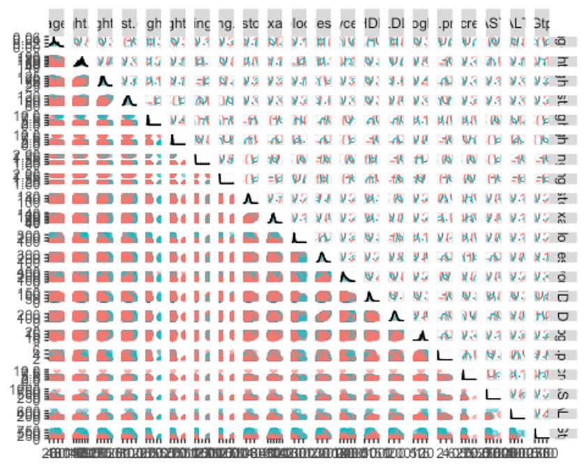
- factor형 변수들의 분포도 확인하자.
ggpairs(df3, columns = c(1, 23, 24, 25), aes(colour = smoking, alpha = 0.4))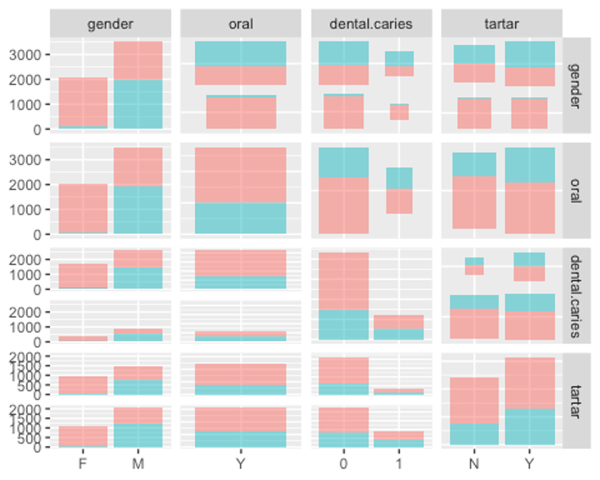
- 이상치가 존재하는지 더 자세히 살펴보기 위해 boxplot을 그려보보자
- 데이터의 범위가 변수별로 차이나므로 평균이 0, 분산이 1이 되도록 스케일링해주고, 데이터를 wide형식에서 long형식으로 바꾼다.
library(reshape2)
library(caret)
model_scale <- preProcess(df_numeric, method = c('center', 'scale'))
scaled_df <- predict(model_scale, df_numeric)
melt_df <- melt(scaled_df, id.vars = 'smoking')
head(melt_df)
##   smoking variable      value
## 1      No      age -1.1768581
## 2      No      age  0.4861341
## 3      No      age -0.7611100
## 4     Yes      age -0.7611100
## 5     Yes      age  1.3176302
## 6 Yes age 0.4861341- boxplot을 그려보자
library(ggplot2)
library(gridExtra)
library(gapminder)
library(dplyr)
##
## Attaching package: 'dplyr'
## The following object is masked from 'package:gridExtra':
##
##     combine
## The following objects are masked from 'package:pastecs':
##
##     first, last
## The following objects are masked from 'package:stats':
##
##     filter, lag
## The following objects are masked from 'package:base':
##
##     intersect, setdiff, setequal, union
p1 <- ggplot(melt_df, aes(x = variable, y = value, fill = smoking)) + geom_boxplot()
p1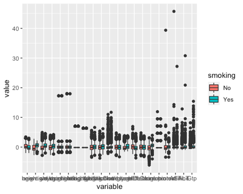
모든 변수에 이상치가 있다.
- 사분위수 99% 범위 밖의 이상치는 75% 사분위수로 바꿔주고, 1%내의 이상치는 25%사분위수로 바꿔준다.
outHigh <- function(x){
  x[x > quantile(x, 0.99)] <- quantile(x, 0.75)
  x
}

outLow <- function(x){
  x[x < quantile(x, 0.01)] <- quantile(x, 0.25)
  x
}

df <- data.frame(lapply(df_numeric[, -22], outHigh))
df <- data.frame(lapply(df, outLow))- 이상치 변경 후의 boxplot을 다시 그려보자
- 이상치를 변경한 데이터를 long형식으로 만든다.
df$smoking <- df3$smoking
scale <- preProcess(df, method = c('center', 'scale'))
scaled <- predict(scale, df)
melt <- melt(scaled, id.vars = 'smoking')
head(melt)
##   smoking variable      value
## 1      No      age -1.1882108
## 2      No      age  0.5028360
## 3      No      age -0.7654491
## 4     Yes      age -0.7654491
## 5     Yes      age  1.3483593
## 6 Yes age 0.5028360- boxplot을 그린다.
p2 <- ggplot(melt, aes(x = variable, y = value, fill = smoking)) + geom_boxplot()
p2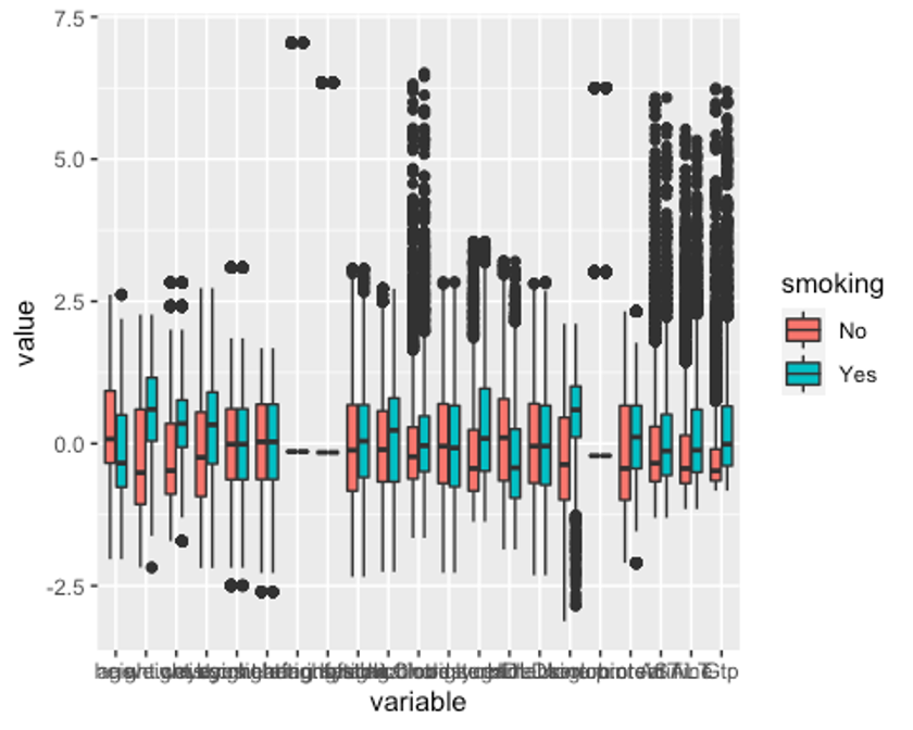
이상치는 잘 교체된 것으로 보인다. 이상치를 교체했는데도 보이는 점들은 현실감있는 데이터를 위해 양 극단의 1%의 이상치만 각각 75%, 25% 사분위수로 바꿨기 때문이다.
- 예측 변수들의 상관관계를 확인해보자.
df_numeric2 <- df_numeric[, -22]
cor_df <- cor(df_numeric2)
library(PerformanceAnalytics)
## Loading required package: xts
## Loading required package: zoo
##
## Attaching package: 'zoo'
## The following objects are masked from 'package:base':
##
##     as.Date, as.Date.numeric
##
## Attaching package: 'xts'
## The following objects are masked from 'package:dplyr':
##
##     first, last
## The following objects are masked from 'package:pastecs':
##
##     first, last
##
## Attaching package: 'PerformanceAnalytics'
## The following object is masked from 'package:graphics':
##
##     legend
chart.Correlation(df_numeric2, histogram = TRUE, pch = 19, method = 'pearson')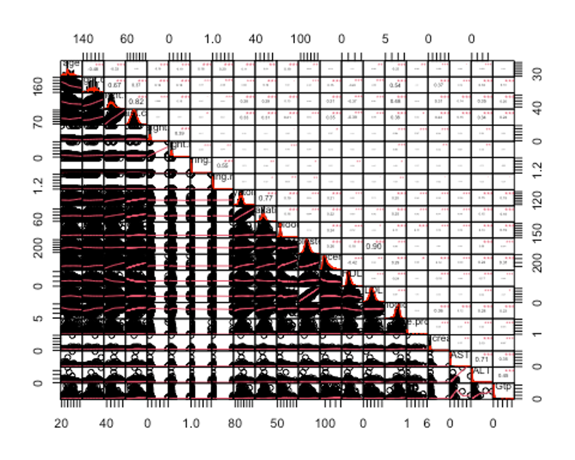
- 상관관계의 값이 0.7이상인 칼럼을 삭제하자.
findCorrelation(cor_df, cutoff = 0.7)
## [1] 3 20 10 15- df_numeric2에서 위의 칼럼을 삭제한다.
new_df <- df_numeric2[, -c(3, 20, 10, 15)]
new_df$gender <- df3$gender
new_df$oral <- df3$oral
new_df$dental.caries <- df3$dental.caries
new_df$tartar <- df3$tartar
new_df$smoking <- df3$smoking
str(new_df)
## 'data.frame':    5570 obs. of  22 variables:
##  $ age                : int  30 50 35 35 60 50 55 50 50 45 ...
##  $ height.cm.         : int  180 150 170 180 160 170 175 150 155 170 ...
##  $ waist.cm.          : num  85 85 84.6 90 91 80 81.5 74.5 73 76 ...
##  $ eyesight.left.     : num  1.2 0.7 1 1.5 0.7 0.9 0.9 0.8 1 1.2 ...
##  $ eyesight.right.    : num  1.2 0.8 1 1.5 0.7 0.9 0.7 0.8 1.2 1.2 ...
##  $ hearing.left.      : num  1 1 1 1 1 1 1 1 1 1 ...
##  $ hearing.right.     : num  1 1 1 1 1 1 1 1 1 1 ...
##  $ systolic           : num  128 115 127 140 130 142 122 110 121 122 ...
##  $ fasting.blood.sugar: num  95 86 87 101 87 91 91 92 122 97 ...
##  $ Cholesterol        : num  217 210 179 191 209 148 223 191 201 170 ...
##  $ triglyceride       : num  199 66 76 218 234 130 108 60 69 108 ...
##  $ HDL                : num  48 48 52 39 30 48 48 80 63 55 ...
##  $ hemoglobin         : num  16.2 13.7 16 17.6 14.7 13.8 16.4 11.6 12.2 13.9 ...
##  $ Urine.protein      : num  1 1 1 1 1 1 1 1 1 1 ...
##  $ serum.creatinine   : num  1.2 0.8 0.8 1 1 1 0.9 0.8 0.9 1 ...
##  $ AST                : num  18 31 16 30 31 43 45 20 17 28 ...
##  $ Gtp                : num  33 14 12 99 70 202 47 8 12 30 ...
##  $ gender             : Factor w/ 2 levels "F","M": 2 1 2 2 2 2 2 1 1 2 ...
##  $ oral               : Factor w/ 1 level "Y": 1 1 1 1 1 1 1 1 1 1 ...
##  $ dental.caries      : Factor w/ 2 levels "0","1": 1 1 1 1 1 1 1 2 1 2 ...
##  $ tartar             : Factor w/ 2 levels "N","Y": 2 1 1 2 1 1 1 2 2 1 ...
## $ smoking : Factor w/ 2 levels "No","Yes": 1 1 1 2 2 2 1 1 1 2 ...- 상관관계가 높은 4개의 예측변수를 삭제했음에도 여전히 예측변수가 21개로 많다. 분산이 0에 가까운 변수는 모델링에 별 도움이 되지 않으므로 마찬가지로 삭제해주자.
nearZeroVar(new_df, saveMetrics = TRUE)
##                     freqRatio percentUnique zeroVar   nzv
## age                  2.278592    0.25134650   FALSE FALSE
## height.cm.           1.121032    0.19748654   FALSE FALSE
## waist.cm.            1.164773    7.36086176   FALSE FALSE
## eyesight.left.       1.045340    0.28725314   FALSE FALSE
## eyesight.right.      1.039409    0.30520646   FALSE FALSE
## hearing.left.       49.636364    0.03590664   FALSE  TRUE
## hearing.right.      40.259259    0.03590664   FALSE  TRUE
## systolic             1.053412    1.81328546   FALSE FALSE
## fasting.blood.sugar  1.101770    2.99820467   FALSE FALSE
## Cholesterol          1.000000    4.02154399   FALSE FALSE
## triglyceride         1.035088    6.40933573   FALSE FALSE
## HDL                  1.085227    1.81328546   FALSE FALSE
## hemoglobin           1.136364    2.06463196   FALSE FALSE
## Urine.protein       28.873626    0.10771993   FALSE  TRUE
## serum.creatinine     1.056903    0.35906643   FALSE FALSE
## AST                  1.010390    2.08258528   FALSE FALSE
## Gtp                  1.009009    4.68581688   FALSE FALSE
## gender               1.710462    0.03590664   FALSE FALSE
## oral                 0.000000    0.01795332    TRUE  TRUE
## dental.caries        3.554374    0.03590664   FALSE FALSE
## tartar               1.291238    0.03590664   FALSE FALSE
## smoking              1.722385    0.03590664   FALSE FALSE
new_df2 <- new_df[, -nearZeroVar(new_df)]
str(new_df2)
## 'data.frame':    5570 obs. of  18 variables:
##  $ age                : int  30 50 35 35 60 50 55 50 50 45 ...
##  $ height.cm.         : int  180 150 170 180 160 170 175 150 155 170 ...
##  $ waist.cm.          : num  85 85 84.6 90 91 80 81.5 74.5 73 76 ...
##  $ eyesight.left.     : num  1.2 0.7 1 1.5 0.7 0.9 0.9 0.8 1 1.2 ...
##  $ eyesight.right.    : num  1.2 0.8 1 1.5 0.7 0.9 0.7 0.8 1.2 1.2 ...
##  $ systolic           : num  128 115 127 140 130 142 122 110 121 122 ...
##  $ fasting.blood.sugar: num  95 86 87 101 87 91 91 92 122 97 ...
##  $ Cholesterol        : num  217 210 179 191 209 148 223 191 201 170 ...
##  $ triglyceride       : num  199 66 76 218 234 130 108 60 69 108 ...
##  $ HDL                : num  48 48 52 39 30 48 48 80 63 55 ...
##  $ hemoglobin         : num  16.2 13.7 16 17.6 14.7 13.8 16.4 11.6 12.2 13.9 ...
##  $ serum.creatinine   : num  1.2 0.8 0.8 1 1 1 0.9 0.8 0.9 1 ...
##  $ AST                : num  18 31 16 30 31 43 45 20 17 28 ...
##  $ Gtp                : num  33 14 12 99 70 202 47 8 12 30 ...
##  $ gender             : Factor w/ 2 levels "F","M": 2 1 2 2 2 2 2 1 1 2 ...
##  $ dental.caries      : Factor w/ 2 levels "0","1": 1 1 1 1 1 1 1 2 1 2 ...
##  $ tartar             : Factor w/ 2 levels "N","Y": 2 1 1 2 1 1 1 2 2 1 ...
##  $ smoking            : Factor w/ 2 levels "No","Yes": 1 1 1 2 2 2 1 1 1 2
분산이 0에 가까운 4개의 변수가 삭제되었다.
- 마지막으로 랜덤포레스트를 사용해 변수를 선택하자.
library(Boruta)
set.seed(123)
feature.selection <- Boruta(smoking ~., data = new_df2, doTrace = 1)
## After 11 iterations, +14 secs:
##  confirmed 10 attributes: age, AST, fasting.blood.sugar, gender, Gtp and 5 more;
##  still have 7 attributes left.
## After 15 iterations, +19 secs:
##  confirmed 2 attributes: Cholesterol, waist.cm.;
##  still have 5 attributes left.
## After 22 iterations, +29 secs:
##  rejected 1 attribute: systolic;
##  still have 4 attributes left.
## After 28 iterations, +37 secs:
##  confirmed 2 attributes: dental.caries, eyesight.left.;
##  still have 2 attributes left.
## After 34 iterations, +45 secs:
##  confirmed 1 attribute: tartar;
##  still have 1 attribute left.
## After 39 iterations, +52 secs:
##  confirmed 1 attribute: eyesight.right.;
##  no more attributes left.
table(feature.selection$finalDecision)
##
## Tentative Confirmed  Rejected
## 0 16 1- 하나의 변수가 Rejected되었다. 삭제하자.
fNames <- getSelectedAttributes(feature.selection, withTentative = TRUE)
final_df <- new_df2[, fNames]
final_df$smoking <- new_df2$smoking
str(final_df)
## 'data.frame':    5570 obs. of  17 variables:
##  $ age                : int  30 50 35 35 60 50 55 50 50 45 ...
##  $ height.cm.         : int  180 150 170 180 160 170 175 150 155 170 ...
##  $ waist.cm.          : num  85 85 84.6 90 91 80 81.5 74.5 73 76 ...
##  $ eyesight.left.     : num  1.2 0.7 1 1.5 0.7 0.9 0.9 0.8 1 1.2 ...
##  $ eyesight.right.    : num  1.2 0.8 1 1.5 0.7 0.9 0.7 0.8 1.2 1.2 ...
##  $ fasting.blood.sugar: num  95 86 87 101 87 91 91 92 122 97 ...
##  $ Cholesterol        : num  217 210 179 191 209 148 223 191 201 170 ...
##  $ triglyceride       : num  199 66 76 218 234 130 108 60 69 108 ...
##  $ HDL                : num  48 48 52 39 30 48 48 80 63 55 ...
##  $ hemoglobin         : num  16.2 13.7 16 17.6 14.7 13.8 16.4 11.6 12.2 13.9 ...
##  $ serum.creatinine   : num  1.2 0.8 0.8 1 1 1 0.9 0.8 0.9 1 ...
##  $ AST                : num  18 31 16 30 31 43 45 20 17 28 ...
##  $ Gtp                : num  33 14 12 99 70 202 47 8 12 30 ...
##  $ gender             : Factor w/ 2 levels "F","M": 2 1 2 2 2 2 2 1 1 2 ...
##  $ dental.caries      : Factor w/ 2 levels "0","1": 1 1 1 1 1 1 1 2 1 2 ...
##  $ tartar             : Factor w/ 2 levels "N","Y": 2 1 1 2 1 1 1 2 2 1 ...
## $ smoking : Factor w/ 2 levels "No","Yes": 1 1 1 2 2 2 1 1 1 2 - 데이터를 train데이터와 test데이터로 분리하자.
idx <- createDataPartition(final_df$smoking, p = 0.7)
train <- final_df[idx$Resample1, ]
test <- final_df[-idx$Resample1, ]
table(train$smoking)
##
##   No  Yes
## 2467 1433
train데이터의 결과변수 smoking이 No가 2467개, Yes가 1433개로 2배 미만의 차이를 보이기 때문에 SMOTE나 ROSE등의 업샘플링을 사용하지는 않겠다.
- 데이터를 스케일링 하자.
model_train <- preProcess(train, method = c('center', 'scale'))
model_test <- preProcess(test, method = c('center', 'scale'))

scaled_train <- predict(model_train, train)
scaled_test <- predict(model_test, test)- 이제 더미변수를 만들어 주자.
dummy1 <- dummyVars(smoking ~., data = train)
train_dummy <- as.data.frame(predict(dummy1, newdata = train))
## Warning in model.frame.default(Terms, newdata, na.action = na.action, xlev =
## object$lvls): variable 'smoking' is not a factor
train_dummy$smoking <- train$smoking

dummy2 <- dummyVars(smoking ~., data = test)
test_dummy <- as.data.frame(predict(dummy2, newdata = test))
## Warning in model.frame.default(Terms, newdata, na.action = na.action, xlev =
## object$lvls): variable 'smoking' is not a factor
test_dummy$smoking <- test$smoking

dummy3 <- dummyVars(smoking ~., data = scaled_train)
scaled_train_dummy <- as.data.frame(predict(dummy3, newdata = scaled_train))
## Warning in model.frame.default(Terms, newdata, na.action = na.action, xlev =
## object$lvls): variable 'smoking' is not a factor
scaled_train_dummy$smoking <- scaled_train$smoking

dummy4 <- dummyVars(smoking ~., data = scaled_test)
scaled_test_dummy <- as.data.frame(predict(dummy4, newdata = scaled_test))
## Warning in model.frame.default(Terms, newdata, na.action = na.action, xlev =
## object$lvls): variable 'smoking' is not a factor
scaled_test_dummy$smoking <- scaled_test$smoking
str(scaled_train_dummy)
## 'data.frame':    3900 obs. of  20 variables:
##  $ age                : num  -1.174 0.486 -0.759 -0.759 0.901 ...
##  $ height.cm.         : num  1.699 -1.61 0.596 1.699 1.148 ...
##  $ waist.cm.          : num  0.2959 0.2959 0.2535 0.8265 -0.0755 ...
##  $ eyesight.left.     : num  0.4142 -0.6753 -0.0216 1.0679 -0.2395 ...
##  $ eyesight.right.    : num  0.41 -0.43 -0.01 1.04 -0.64 ...
##  $ fasting.blood.sugar: num  -0.2191 -0.5938 -0.5522 0.0307 -0.3856 ...
##  $ Cholesterol        : num  0.566 0.374 -0.478 -0.148 0.731 ...
##  $ triglyceride       : num  1.013 -0.856 -0.716 1.28 -0.266 ...
##  $ HDL                : num  -0.613 -0.613 -0.333 -1.242 -0.613 ...
##  $ hemoglobin         : num  0.997 -0.562 0.872 1.87 1.122 ...
##  $ serum.creatinine   : num  1.2824 -0.3383 -0.3383 0.4721 0.0669 ...
##  $ AST                : num  -0.464 0.269 -0.577 0.213 1.058 ...
##  $ Gtp                : num  -0.147 -0.498 -0.535 1.074 0.112 ...
##  $ gender.F           : num  0 1 0 0 0 1 1 0 0 1 ...
##  $ gender.M           : num  1 0 1 1 1 0 0 1 1 0 ...
##  $ dental.caries.0    : num  1 1 1 1 1 0 1 0 0 1 ...
##  $ dental.caries.1    : num  0 0 0 0 0 1 0 1 1 0 ...
##  $ tartar.N           : num  0 1 1 0 1 0 0 1 0 0 ...
##  $ tartar.Y           : num  1 0 0 1 0 1 1 0 1 1 ...
##  $ smoking            : Factor w/ 2 levels "No","Yes": 1 1 1 2 1 1 1 2 2 1 ...
세트 1 - train, test : 데이터 스케일X, 더미변수X
세트 2 - scaled_train, scaled_test : 데이터 스케일O, 더미변수X
세트 3 - train_dummy, test_dummy : 데이터 스케일X, 더미변수O
세트 4 - scaled_train_dummy, scaled_test_dummy : 데이터 스케일O, 더미변수O
이렇게 총 4개의 데이터 세트로 모델훈련법에 따라 데이터 세트를 선택해서 사용한다.
다변량 적응 회귀 스플라인(MARS)
- train, test데이터를 사용한다.
library(earth)
## Loading required package: Formula
## Loading required package: plotmo
## Loading required package: plotrix
##
## Attaching package: 'plotrix'
## The following object is masked from 'package:psych':
##
##     rescale
## Loading required package: TeachingDemos
set.seed(123)
earth.fit <- earth(smoking ~., data = train,
                   pmethod = 'cv', nfold = 5,
                   ncross = 3, degree = 1,
                   minspan = -1,
                   glm = list(family = binomial))
summary(earth.fit)
## Call: earth(formula=smoking~., data=train, pmethod="cv",
##             glm=list(family=binomial), degree=1, nfold=5, ncross=3, minspan=-1)
##
## GLM coefficients
##                                  Yes
## (Intercept)               -4.7399931
## Gtp                        0.0725835
## genderM                    3.2050846
## tartarY                    0.2990772
## h(40-age)                 -0.0411159
## h(age-40)                 -0.0284079
## h(82-waist.cm.)            0.0406381
## h(96-fasting.blood.sugar)  0.0179840
## h(fasting.blood.sugar-96)  0.0036683
## h(108-triglyceride)       -0.0089880
## h(triglyceride-108)        0.0009176
## h(hemoglobin-14.8)         0.1142071
## h(0.9-serum.creatinine)    0.3416436
## h(serum.creatinine-0.9)   -1.5411033
## h(23-AST)                  0.0413212
## h(AST-23)                 -0.0053351
## h(Gtp-26)                 -0.0672622
##
## GLM (family binomial, link logit):
##  nulldev   df       dev   df   devratio     AIC iters converged
##   5129.1 3899   3646.12 3883      0.289    3680     5         1
##
## Earth selected 17 of 19 terms, and 10 of 16 predictors (pmethod="cv")
## Termination condition: RSq changed by less than 0.001 at 19 terms
## Importance: genderM, Gtp, age, triglyceride, serum.creatinine, tartarY, ...
## Number of terms at each degree of interaction: 1 16 (additive model)
## Earth GRSq 0.3004701  RSq 0.3119054  mean.oof.RSq 0.2943407 (sd 0.0223)
##
## pmethod="backward" would have selected:
##     12 terms 9 preds,  GRSq 0.3016702  RSq 0.3095286  mean.oof.RSq 0.2937606
위의 코드에서 pmethod = ‘cv’, nfold = 5를 통해 5겹 교차검증의 모형 선택을 명시하고, ncross = 3으로 반복은 3회, degree = 1로 상호작용항 없이 가산모형을 쓰고, mispan = -1로 힌지는 입력 피처 하나당 1개만 사용했다.
또한 이 모형은 절편과 11개의 예측변수를 포함, 총 12개의 항을 갖는다. 예측변수 중 8개는 힌지 함수를 갖는다.
- plotmo()함수를 이용해 해당 예측 변수를 변화시키고 다른 변수들은 상수로 유지했을 때, 모형의 반응 변수가 변하는 양상을 보자.
par("mar")
## [1] 5.1 4.1 4.1 2.1
par(mar=c(1,1,1,1))
plotmo(earth.fit)
##  plotmo grid:    age height.cm. waist.cm. eyesight.left. eyesight.right.
##                   40        165        82              1               1
##  fasting.blood.sugar Cholesterol triglyceride HDL hemoglobin serum.creatinine
##                   96         194          108  55       14.8              0.9
##  AST Gtp gender dental.caries tartar
##   23  26      M             0      Y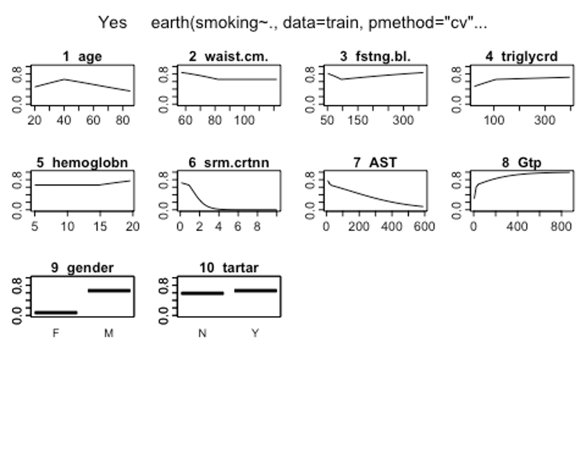
- plotd()함수를 이용해 클래스 라벨에 따른 예측 확률의 밀도 함수 도표를 보자.
plotd(earth.fit)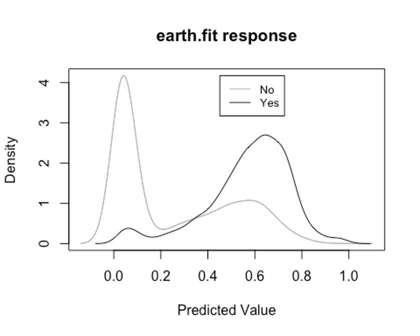
- evimp()함수로 상대적인 변수의 중요도를 보자.
- nsubsets하는 변수명을 볼 수 있는데, 이는 가지치기 패스를 한 후에 남는 변수를 담고 있는 모형의 서브세트 개수이다.
- gcv와 rss칼럼은 각 예측변수가 기여하는 각 감소값을 나타낸다.
evimp(earth.fit)
##                     nsubsets   gcv    rss
## genderM                   16 100.0  100.0
## Gtp                       15  37.8   41.4
## age                       14  29.7   34.2
## triglyceride              11  16.3   22.5
## serum.creatinine          10  12.4   19.4
## tartarY                    9   8.7   16.7
## hemoglobin                 8   6.0   14.7
## waist.cm.                  7   2.6   12.9
## AST                        6  -4.5   10.8
## fasting.blood.sugar        5  -6.3    8.7
16개의 예측변수 중 10개의 예측변수가 선택되었고, 그 중 상대적으로 중요한 변수는 gender, Gtp, age, triglyceride, serum.creatinine순으로 나타났다.
- 이제 test세트에 관해 모형이 얼마나 잘 작동하는지 알아보자.
test.earth.fit <- predict(earth.fit, newdata = test, type = 'class')
head(test.earth.fit)
##      Yes
## [1,] "Yes"
## [2,] "Yes"
## [3,] "Yes"
## [4,] "Yes"
## [5,] "Yes"
## [6,] "Yes"
test.earth.fit <- as.factor(test.earth.fit)

earth.confusion <- confusionMatrix(test.earth.fit, test$smoking, positive = 'Yes')
earth.confusion
## Confusion Matrix and Statistics
##
##           Reference
## Prediction  No Yes
##        No  827 169
##        Yes 230 444
##
##                Accuracy : 0.7611
##                  95% CI : (0.7399, 0.7814)
##     No Information Rate : 0.6329
##     P-Value [Acc > NIR] : < 2.2e-16
##
##                   Kappa : 0.4963
##
##  Mcnemar's Test P-Value : 0.002667
##
##             Sensitivity : 0.7243
##             Specificity : 0.7824
##          Pos Pred Value : 0.6588
##          Neg Pred Value : 0.8303
##              Prevalence : 0.3671
##          Detection Rate : 0.2659
##    Detection Prevalence : 0.4036
##       Balanced Accuracy : 0.7534
##
##        'Positive' Class : Yes
##
earth.confusion$byClass
##          Sensitivity          Specificity       Pos Pred Value
##            0.7243067            0.7824030            0.6587537
##       Neg Pred Value            Precision               Recall
##            0.8303213            0.6587537            0.7243067
##                   F1           Prevalence       Detection Rate
##            0.6899767            0.3670659            0.2658683
## Detection Prevalence    Balanced Accuracy
##            0.4035928            0.7533549
MARS모델의 Accuracy는 0.7611이고, 카파통계량은 0.4963, F1 score는 0.6899767이다.
- 다음으로 ROC커브를 그려보자.
library(ROCR)
test.earth.pred <- predict(earth.fit, newdata = test, type = 'response')
head(test.earth.pred)
##            Yes
## [1,] 0.5247097
## [2,] 0.7181490
## [3,] 0.8198495
## [4,] 0.5000105
## [5,] 0.7135809
## [6,] 0.6827555
pred.earth <- prediction(test.earth.pred, test$smoking)
perf.earth <- performance(pred.earth, 'tpr', 'fpr')
plot(perf.earth, col = 1)
legend(0.6, 0.6, c('MARS'), 1)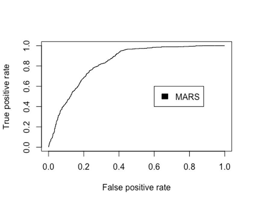
- AUC를 확인해보자.
performance(pred.earth, 'auc')@y.values
## [[1]]
## [1] 0.8359002
MARS모델의 Accuracy는 0.761이고, 카파통계량은 0.496, F1 score는 0.690, AUC는 0.836로 나타났다.
KNN
- K-최근접 이웃법을 이용해 모델링을 해보자.
- scaled_train_dummy, scaled_test_dummy데이터를 사용한다.
- 필요한 패키지들을 불러오자
library(class)
library(kknn)
##
## Attaching package: 'kknn'
## The following object is masked from 'package:caret':
##
##     contr.dummy
library(e1071)
##
## Attaching package: 'e1071'
## The following objects are masked from 'package:PerformanceAnalytics':
##
##     kurtosis, skewness
library(MASS)
##
## Attaching package: 'MASS'
## The following object is masked from 'package:dplyr':
##
##     select
library(kernlab)
##
## Attaching package: 'kernlab'
## The following object is masked from 'package:psych':
##
##     alpha
## The following object is masked from 'package:ggplot2':
##
##     alpha
library(corrplot)
## corrplot 0.92 loaded- KNN을 사용할 때는 적절한 k를 선택하는 일이 매우 중요하다. expand.grid()와 seq()함수를 사용해 보자.
grid1 <- expand.grid(.k = seq(2, 30, by = 1))
control <- trainControl(method = 'cv')
set.seed(123)
knn.train <- train(smoking ~., data = scaled_train_dummy,
                   method = 'knn',
                   trControl = control,
                   tuneGrid = grid1)
knn.train
## k-Nearest Neighbors
##
## 3900 samples
##   19 predictor
##    2 classes: 'No', 'Yes'
##
## No pre-processing
## Resampling: Cross-Validated (10 fold)
## Summary of sample sizes: 3509, 3510, 3509, 3511, 3510, 3511, ...
## Resampling results across tuning parameters:
##
##   k   Accuracy   Kappa
##    2  0.6789665  0.3053793
##    3  0.6969147  0.3477000
##    4  0.6902427  0.3306808
##    5  0.7020436  0.3623090
##    6  0.7017865  0.3595659
##    7  0.7089634  0.3762873
##    8  0.7023111  0.3638328
##    9  0.7089686  0.3782385
##   10  0.7143677  0.3884254
##   11  0.7151304  0.3923099
##   12  0.7125630  0.3858971
##   13  0.7156445  0.3947467
##   14  0.7140988  0.3908974
##   15  0.7110357  0.3840640
##   16  0.7143500  0.3923475
##   17  0.7176833  0.3986310
##   18  0.7197425  0.4028696
##   19  0.7189654  0.3999039
##   20  0.7204999  0.4025669
##   21  0.7251238  0.4136475
##   22  0.7228155  0.4104596
##   23  0.7292185  0.4226905
##   24  0.7274283  0.4207804
##   25  0.7233309  0.4085841
##   26  0.7207714  0.4048223
##   27  0.7235853  0.4086007
##   28  0.7274296  0.4180632
##   29  0.7256393  0.4140248
##   30  0.7238398  0.4101515
##
## Accuracy was used to select the optimal model using the largest value.
## The final value used for the model was k = 23.
k매개변수 값으로 23이 나왔다.
- knn()함수를 이용해 모델을 만들어 보자.
knn.model <- knn(scaled_train_dummy[, -20], scaled_test_dummy[, -20], scaled_train_dummy[, 20], k = 23)
summary(knn.model)
##   No  Yes
## 1042 628- scaled_test_dummy를 이용해 모형이 얼마나 잘 작동하는지 보자.
knn.confusion <- confusionMatrix(knn.model, scaled_test_dummy$smoking, positive = 'Yes')
knn.confusion
## Confusion Matrix and Statistics
##
##           Reference
## Prediction  No Yes
##        No  818 224
##        Yes 239 389
##
##                Accuracy : 0.7228
##                  95% CI : (0.7006, 0.7441)
##     No Information Rate : 0.6329
##     P-Value [Acc > NIR] : 4.694e-15
##
##                   Kappa : 0.4064
##
##  Mcnemar's Test P-Value : 0.5153
##
##             Sensitivity : 0.6346
##             Specificity : 0.7739
##          Pos Pred Value : 0.6194
##          Neg Pred Value : 0.7850
##              Prevalence : 0.3671
##          Detection Rate : 0.2329
##    Detection Prevalence : 0.3760
##       Balanced Accuracy : 0.7042
##
##        'Positive' Class : Yes
##
knn.confusion$byClass
##          Sensitivity          Specificity       Pos Pred Value
##            0.6345840            0.7738884            0.6194268
##       Neg Pred Value            Precision               Recall
##            0.7850288            0.6194268            0.6345840
##                   F1           Prevalence       Detection Rate
##            0.6269138            0.3670659            0.2329341
## Detection Prevalence    Balanced Accuracy
##            0.3760479            0.7042362
knn모델의 Accuracy는 0.723, kappa통계량은 0.408, F1 score는 0.628로 MARS모델보다 성능이 떨어진다.
- 성능을 올리기 위해 커널을 입력하자.
- distance = 2로 설정해 절댓값합 거리를 사용하자.
kknn.train <- train.kknn(smoking ~., data = scaled_train_dummy,
                         kmax = 30, distance = 2,
                         kernel = c('rectangular', 'triangular', 'epanechnikov'))
plot(kknn.train)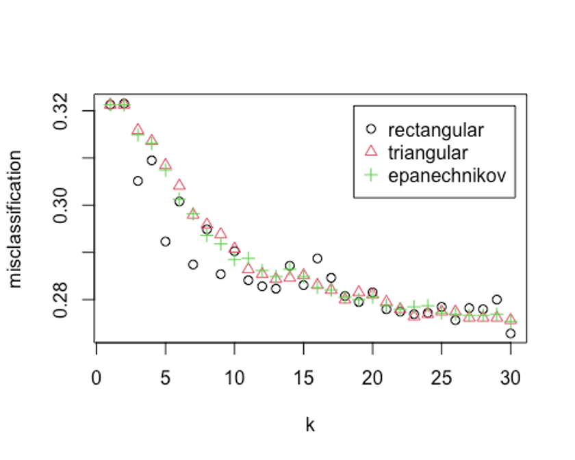
kknn.train
##
## Call:
## train.kknn(formula = smoking ~ ., data = scaled_train_dummy,     kmax = 30, distance = 2, kernel = c("rectangular", "triangular",         "epanechnikov"))
##
## Type of response variable: nominal
## Minimal misclassification: 0.2728205
## Best kernel: rectangular
## Best k: 30
k = 30, rectangular커널을 사용했을 때 가장 오류가 낮다.
- 예측 성능을 보자.
kknn.fit <- predict(kknn.train, newdata = scaled_test_dummy)
kknn.fit <- as.factor(kknn.fit)
kknn.confusion <- confusionMatrix(kknn.fit, scaled_test_dummy$smoking, positive = 'Yes')
kknn.confusion
## Confusion Matrix and Statistics
##
##           Reference
## Prediction  No Yes
##        No  816 185
##        Yes 241 428
##
##                Accuracy : 0.7449
##                  95% CI : (0.7233, 0.7657)
##     No Information Rate : 0.6329
##     P-Value [Acc > NIR] : < 2.2e-16
##
##                   Kappa : 0.4613
##
##  Mcnemar's Test P-Value : 0.007704
##
##             Sensitivity : 0.6982
##             Specificity : 0.7720
##          Pos Pred Value : 0.6398
##          Neg Pred Value : 0.8152
##              Prevalence : 0.3671
##          Detection Rate : 0.2563
##    Detection Prevalence : 0.4006
##       Balanced Accuracy : 0.7351
##
##        'Positive' Class : Yes
##
kknn.confusion$byClass
##          Sensitivity          Specificity       Pos Pred Value
##            0.6982055            0.7719962            0.6397608
##       Neg Pred Value            Precision               Recall
##            0.8151848            0.6397608            0.6982055
##                   F1           Prevalence       Detection Rate
##            0.6677067            0.3670659            0.2562874
## Detection Prevalence    Balanced Accuracy
##            0.4005988            0.7351009
Accuracy는 0.745, kappa통계량은 0.461, F1 score는 0.668이다.
- ROC커브를 그려보자.
plot(perf.earth, col = 1)
knn.pred <- predict(kknn.train, newdata = scaled_test_dummy, type = 'prob')
head(knn.pred)
##             No       Yes
## [1,] 0.2000000 0.8000000
## [2,] 0.3666667 0.6333333
## [3,] 0.2666667 0.7333333
## [4,] 0.3333333 0.6666667
## [5,] 0.1666667 0.8333333
## [6,] 0.4333333 0.5666667
knn.pred.yes <- knn.pred[, 2]
pred.knn <- prediction(knn.pred.yes, scaled_test_dummy$smoking)
perf.knn <- performance(pred.knn, 'tpr', 'fpr')
plot(perf.knn, col = 2, add = TRUE)
legend(0.6, 0.6, c('MARS', 'KNN'), 1:2)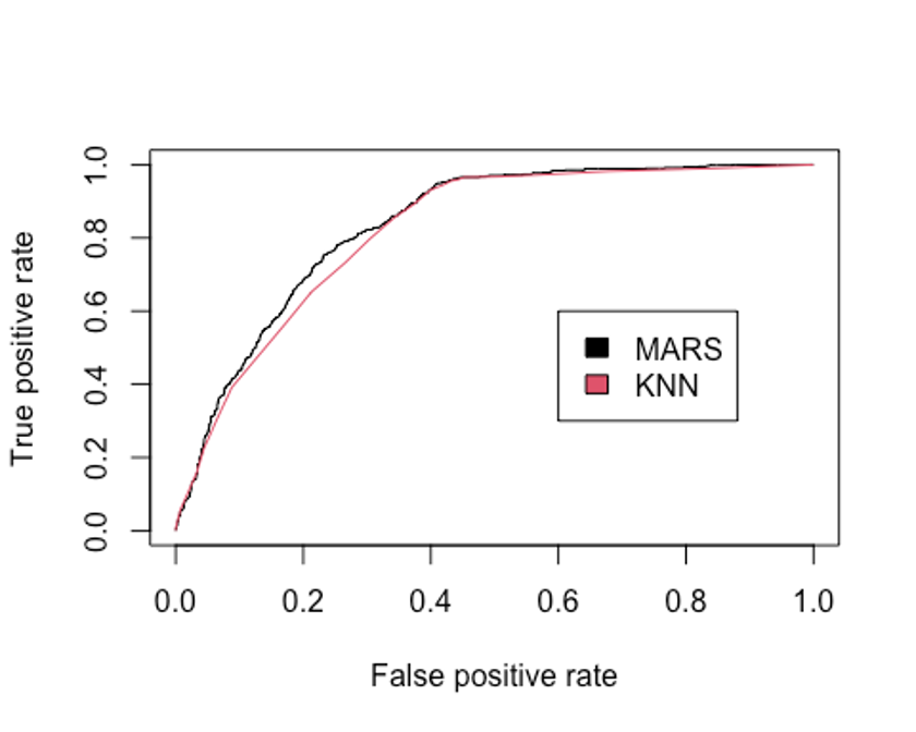
- KNN모델의 AUC를 알아보자
performance(pred.knn, 'auc')@y.values
## [[1]]
## [1] 0.8207136
KNN모델의 Accuracy는 0.745, kappa통계량은 0.461, F1 score는 0.668, AUC는 0.821로 MARS모델(Accuracy = 0.761, 카파통계량 = 0.496, F1 score = 0.690, AUC = 0.836)에 비해 성능이 떨어진다.
SVM
- 다음으로 SVM을 이용해 보자.
- scaled_train, scaled_test데이터를 사용하자.
- 선형 SVM분류기부터 시작해보자.
- tune.svm함수를 사용해 튜닝 파라미터 및 커널 함수를 선택하자.
linear.tune <- tune.svm(smoking ~., data = scaled_train,
                        kernel = 'linear',
                        cost = c(0.001, 0.01, 0.1, 0.5, 1, 2, 5, 10))
summary(linear.tune)
##
## Parameter tuning of 'svm':
##
## - sampling method: 10-fold cross validation
##
## - best parameters:
##  cost
##   0.5
##
## - best performance: 0.2725641
##
## - Detailed performance results:
##    cost     error dispersion
## 1 1e-03 0.2861538 0.02073244
## 2 1e-02 0.2758974 0.01845837
## 3 1e-01 0.2730769 0.02062824
## 4 5e-01 0.2725641 0.02169156
## 5 1e+00 0.2741026 0.02278864
## 6 2e+00 0.2741026 0.02246579
## 7 5e+00 0.2743590 0.02199091
## 8 1e+01 0.2741026 0.02226984
이 문제에서 최적의 cost함수는 0.5로 나왔고, 분류 오류 비율은 대략 27.538% 정도이다.
- predict()함수로 scaled_test데이터 예측을 실행해보자.
best.linear <- linear.tune$best.model
tune.fit <- predict(best.linear, newdata = scaled_test, type = 'class')
tune.fit <- as.factor(tune.fit)
linear.svm.confusion <- confusionMatrix(tune.fit, scaled_test$smoking, positive = 'Yes')
linear.svm.confusion
## Confusion Matrix and Statistics
##
##           Reference
## Prediction  No Yes
##        No  754 143
##        Yes 303 470
##
##                Accuracy : 0.7329
##                  95% CI : (0.711, 0.754)
##     No Information Rate : 0.6329
##     P-Value [Acc > NIR] : < 2.2e-16
##
##                   Kappa : 0.4551
##
##  Mcnemar's Test P-Value : 5.118e-14
##
##             Sensitivity : 0.7667
##             Specificity : 0.7133
##          Pos Pred Value : 0.6080
##          Neg Pred Value : 0.8406
##              Prevalence : 0.3671
##          Detection Rate : 0.2814
##    Detection Prevalence : 0.4629
##       Balanced Accuracy : 0.7400
##
##        'Positive' Class : Yes
##
linear.svm.confusion$byClass
##          Sensitivity          Specificity       Pos Pred Value
##            0.7667210            0.7133396            0.6080207
##       Neg Pred Value            Precision               Recall
##            0.8405797            0.6080207            0.7667210
##                   F1           Prevalence       Detection Rate
##            0.6782107            0.3670659            0.2814371
## Detection Prevalence    Balanced Accuracy
##            0.4628743            0.7400303
Accuracy는 0.7329, 카파통계량은 0.4551, F1 score는 0.678로 MARS모델보다 성능이 떨어진다.
- 비선형 방법을 이용해 성능을 더 높혀보자.
- 먼저 polynomial커널함수를 적용해보자.
- ploynimial의 차수는 3, 4, 5의 값을 주고, 커널 계수는 0.1부터 4의 수를 준다.
set.seed(123)
poly.tune <- tune.svm(smoking ~., data = scaled_train,
                      kernel = 'polynomial', degree = c(3, 4, 5),
                      coef0 = c(0.1, 0.5, 1, 2, 3, 4))
summary(poly.tune)
##
## Parameter tuning of 'svm':
##
## - sampling method: 10-fold cross validation
##
## - best parameters:
##  degree coef0
##       3     2
##
## - best performance: 0.2597436
##
## - Detailed performance results:
##    degree coef0     error dispersion
## 1       3   0.1 0.2664103 0.01672464
## 2       4   0.1 0.2830769 0.01877231
## 3       5   0.1 0.3133333 0.02085890
## 4       3   0.5 0.2623077 0.01926587
## 5       4   0.5 0.2615385 0.01635139
## 6       5   0.5 0.2617949 0.01736747
## 7       3   1.0 0.2607692 0.01784872
## 8       4   1.0 0.2671795 0.01978037
## 9       5   1.0 0.2656410 0.01793650
## 10      3   2.0 0.2597436 0.01470731
## 11      4   2.0 0.2702564 0.01813900
## 12      5   2.0 0.2751282 0.01670716
## 13      3   3.0 0.2633333 0.01313295
## 14      4   3.0 0.2682051 0.01946017
## 15      5   3.0 0.2900000 0.01961906
## 16      3   4.0 0.2646154 0.01243289
## 17      4   4.0 0.2676923 0.01515498
## 18      5   4.0 0.2953846 0.01750781
이 모형은 다항식의 차수 degree의 값으로 3, 커널계수는 2를 선택했다.
- scaled_test데이터로 예측을 해보자
best.poly <- poly.tune$best.model
poly.test <- predict(best.poly, newdata = scaled_test, type = 'class')
poly.test <- as.factor(poly.test)
poly.svm.confusion <- confusionMatrix(poly.test, scaled_test$smoking, positive = 'Yes')
poly.svm.confusion
## Confusion Matrix and Statistics
##
##           Reference
## Prediction  No Yes
##        No  826 195
##        Yes 231 418
##
##                Accuracy : 0.7449
##                  95% CI : (0.7233, 0.7657)
##     No Information Rate : 0.6329
##     P-Value [Acc > NIR] : < 2e-16
##
##                   Kappa : 0.4577
##
##  Mcnemar's Test P-Value : 0.08993
##
##             Sensitivity : 0.6819
##             Specificity : 0.7815
##          Pos Pred Value : 0.6441
##          Neg Pred Value : 0.8090
##              Prevalence : 0.3671
##          Detection Rate : 0.2503
##    Detection Prevalence : 0.3886
##       Balanced Accuracy : 0.7317
##
##        'Positive' Class : Yes
##
poly.svm.confusion$byClass
##          Sensitivity          Specificity       Pos Pred Value
##            0.6818923            0.7814570            0.6440678
##       Neg Pred Value            Precision               Recall
##            0.8090108            0.6440678            0.6818923
##                   F1           Prevalence       Detection Rate
##            0.6624406            0.3670659            0.2502994
## Detection Prevalence    Balanced Accuracy
##            0.3886228            0.7316746
커널함수로 polynomial을 설정한 SVM모델은 Accuracy : 0.745, 카파통계량 0.458, F1 score는 0.662로 선형SVM의 성능(Accuracy = 0.733, 카파통계량 = 0.455, F1 score = 0.678)과 거의 유사한 성능을 보인다.
- 다음으로 방사 기저 함수를 커널로 설정해보자
- 매개변수는 gamma로 최적값을 찾기 위해 0.1부터 4까지 증가시켜 본다.
- gamma값이 너무 작을 때는 모형이 결정분계선을 제대로 포착하지 못할 수 있고, 값이 너무 클 때는 모형이 지나치게 과적합될 수 있으므로 주의가 필요하다.
set.seed(123)
rbf.tune <- tune.svm(smoking ~., data = scaled_train,
                     kernel = 'radial',
                     gamma = c(0.1, 0.5, 1, 2, 3, 4))
summary(rbf.tune)
##
## Parameter tuning of 'svm':
##
## - sampling method: 10-fold cross validation
##
## - best parameters:
##  gamma
##    0.1
##
## - best performance: 0.2597436
##
## - Detailed performance results:
##   gamma     error dispersion
## 1   0.1 0.2597436 0.01718140
## 2   0.5 0.2902564 0.01944515
## 3   1.0 0.3410256 0.02834722
## 4   2.0 0.3610256 0.03023757
## 5   3.0 0.3612821 0.03039781
## 6   4.0 0.3612821 0.03039781
최적의 gamma 값은 0.1이다.
- 마찬가지로 성능을 예측해보자.
best.rbf <- rbf.tune$best.model
rbf.test <- predict(best.rbf, newdata = scaled_test, type = 'class')
rbf.test <- as.factor(rbf.test)
rbf.svm.confusion <- confusionMatrix(rbf.test, scaled_test$smoking, positive = 'Yes')
rbf.svm.confusion
## Confusion Matrix and Statistics
##
##           Reference
## Prediction  No Yes
##        No  835 208
##        Yes 222 405
##
##                Accuracy : 0.7425
##                  95% CI : (0.7208, 0.7633)
##     No Information Rate : 0.6329
##     P-Value [Acc > NIR] : <2e-16
##
##                   Kappa : 0.4485
##
##  Mcnemar's Test P-Value : 0.5307
##
##             Sensitivity : 0.6607
##             Specificity : 0.7900
##          Pos Pred Value : 0.6459
##          Neg Pred Value : 0.8006
##              Prevalence : 0.3671
##          Detection Rate : 0.2425
##    Detection Prevalence : 0.3754
##       Balanced Accuracy : 0.7253
##
##        'Positive' Class : Yes
##
rbf.svm.confusion$byClass
##          Sensitivity          Specificity       Pos Pred Value
##            0.6606852            0.7899716            0.6459330
##       Neg Pred Value            Precision               Recall
##            0.8005753            0.6459330            0.6606852
##                   F1           Prevalence       Detection Rate
##            0.6532258            0.3670659            0.2425150
## Detection Prevalence    Balanced Accuracy
##            0.3754491            0.7253284
Accuracy : 0.743, 카파통계량 0.449, F1 score는 0.653으로 polynomial을 설정한 SVM모델의 성능(Accuracy = 0.745, 카파통계량 = 0.458, F1 score = 0.662)보다 오히려 살짝 낮은 성능을 보인다.
- 다시 성능 개선을 위해 커널 함수를 sigmoid함수로 설정해보자.
- 매개변수인 gamma와 coef0이 최적의 값이 되도록 계산해보자.
set.seed(123)
sigmoid.tune <- tune.svm(smoking ~., data = scaled_train,
                         kernel = 'sigmoid',
                         gamma = c(0.1, 0.5, 1, 2, 3, 4),
                         coef0 = c(0.1, 0.5, 1, 2, 3, 4))
summary(sigmoid.tune)
##
## Parameter tuning of 'svm':
##
## - sampling method: 10-fold cross validation
##
## - best parameters:
##  gamma coef0
##    0.1   0.1
##
## - best performance: 0.355641
##
## - Detailed performance results:
##    gamma coef0     error dispersion
## 1    0.1   0.1 0.3556410 0.01837309
## 2    0.5   0.1 0.3733333 0.02216297
## 3    1.0   0.1 0.3761538 0.02004633
## 4    2.0   0.1 0.3758974 0.02738246
## 5    3.0   0.1 0.3779487 0.02492446
## 6    4.0   0.1 0.3789744 0.02336947
## 7    0.1   0.5 0.3587179 0.01632680
## 8    0.5   0.5 0.3894872 0.02754869
## 9    1.0   0.5 0.3910256 0.01773376
## 10   2.0   0.5 0.3820513 0.02097067
## 11   3.0   0.5 0.3887179 0.01567625
## 12   4.0   0.5 0.3841026 0.02311804
## 13   0.1   1.0 0.3702564 0.01599912
## 14   0.5   1.0 0.3887179 0.02819736
## 15   1.0   1.0 0.3992308 0.02258255
## 16   2.0   1.0 0.3771795 0.01596484
## 17   3.0   1.0 0.3782051 0.02381688
## 18   4.0   1.0 0.3843590 0.01502184
## 19   0.1   2.0 0.3874359 0.01786509
## 20   0.5   2.0 0.4076923 0.02438520
## 21   1.0   2.0 0.4200000 0.02597503
## 22   2.0   2.0 0.3912821 0.01927156
## 23   3.0   2.0 0.3853846 0.02179236
## 24   4.0   2.0 0.3776923 0.01801169
## 25   0.1   3.0 0.3592308 0.02493179
## 26   0.5   3.0 0.4374359 0.02598628
## 27   1.0   3.0 0.4089744 0.02498447
## 28   2.0   3.0 0.3910256 0.02539051
## 29   3.0   3.0 0.3869231 0.01770077
## 30   4.0   3.0 0.3856410 0.02132303
## 31   0.1   4.0 0.4053846 0.02682318
## 32   0.5   4.0 0.4428205 0.02575615
## 33   1.0   4.0 0.4200000 0.02014630
## 34   2.0   4.0 0.3948718 0.02515203
## 35   3.0   4.0 0.3843590 0.02373084
## 36   4.0   4.0 0.3938462 0.02115104
최적의 gamma값은 0.1이고, coef0값은 0.1이다.
- 예측을 해보자
best.sigmoid <- sigmoid.tune$best.model
sigmoid.test <- predict(best.sigmoid, newdata = scaled_test, type = 'class')
sigmoid.test <- as.factor(sigmoid.test)
sigmoid.svm.confusion <- confusionMatrix(sigmoid.test, scaled_test$smoking, positive = 'Yes')
sigmoid.svm.confusion
## Confusion Matrix and Statistics
##
##           Reference
## Prediction  No Yes
##        No  775 311
##        Yes 282 302
##
##                Accuracy : 0.6449
##                  95% CI : (0.6214, 0.6679)
##     No Information Rate : 0.6329
##     P-Value [Acc > NIR] : 0.1611
##
##                   Kappa : 0.2281
##
##  Mcnemar's Test P-Value : 0.2502
##
##             Sensitivity : 0.4927
##             Specificity : 0.7332
##          Pos Pred Value : 0.5171
##          Neg Pred Value : 0.7136
##              Prevalence : 0.3671
##          Detection Rate : 0.1808
##    Detection Prevalence : 0.3497
##       Balanced Accuracy : 0.6129
##
##        'Positive' Class : Yes
##
sigmoid.svm.confusion$byClass
##          Sensitivity          Specificity       Pos Pred Value
##            0.4926591            0.7332072            0.5171233
##       Neg Pred Value            Precision               Recall
##            0.7136280            0.5171233            0.4926591
##                   F1           Prevalence       Detection Rate
##            0.5045948            0.3670659            0.1808383
## Detection Prevalence    Balanced Accuracy
##            0.3497006            0.6129331
Accuracy는 0.6449, 카파통계량은 0.2281, F1 score는 0.505로 시그모이드 커널 모형이 SVM모형 중 가장 나쁜 성능을 보였다. F1 score를 기준으로 SVM 모형 중 선형모형이 가장 높은 F1 score를 기록했다. 따라서 지금의 데이터로는 SVM에서 커널 함수가 성능을 올리지 못하는 것으로 보인다.
- 선형 SVM모델의 ROC커브를 그려보자.
plot(perf.earth, col = 1)
plot(perf.knn, col = 2, add = TRUE)

linear.svm <- svm(smoking ~., data=scaled_train, kernel="linear", cost = 0.5, scale=FALSE, probability=TRUE)
pred_svm <- predict(linear.svm, scaled_test, probability=TRUE)
prob <- attr(pred_svm,"probabilities")

pred.svm <- prediction(prob[, 2], scaled_test$smoking)
perf.svm <- performance(pred.svm, 'tpr', 'fpr')
plot(perf.svm, col = 3, add = TRUE)
legend(0.6, 0.6, c('MARS', 'KNN', 'SVM'), 1:3)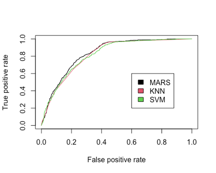
- 선형 SVM 분류기의 AUC를 알아보자.
performance(pred.earth, 'auc')@y.values
## [[1]]
## [1] 0.8359002
performance(pred.knn, 'auc')@y.values
## [[1]]
## [1] 0.8207136
performance(pred.svm, 'auc')@y.values
## [[1]]
## [1] 0.82103
지금까지 만든 모형중 AUC를 성능 기준으로 삼는다면 MARS모형이 가장 좋은 성능을 보였고, 그 다음으로 SVM이 좋은 성능을 보이고 있다.
랜덤포레스트
- 랜덤포레스트를 사용해 모델을 만들어보자.
- train, test데이터를 사용한다.
- 필요한 패키지를 불러오자.
library(rpart)
library(partykit)
## Loading required package: grid
## Loading required package: libcoin
## Loading required package: mvtnorm
library(MASS)
library(genridge)
## Loading required package: car
## Loading required package: carData
##
## Attaching package: 'car'
## The following object is masked from 'package:dplyr':
##
##     recode
## The following object is masked from 'package:psych':
##
##     logit
##
## Attaching package: 'genridge'
## The following object is masked from 'package:caret':
##
##     precision
library(randomForest)
## randomForest 4.7-1
## Type rfNews() to see new features/changes/bug fixes.
##
## Attaching package: 'randomForest'
## The following object is masked from 'package:dplyr':
##
##     combine
## The following object is masked from 'package:gridExtra':
##
##     combine
## The following object is masked from 'package:psych':
##
##     outlier
## The following object is masked from 'package:ggplot2':
##
##     margin
library(xgboost)
##
## Attaching package: 'xgboost'
## The following object is masked from 'package:dplyr':
##
## slice- 기본 모형을 만들어 보자.
set.seed(123)
rf.model <- randomForest(smoking ~., data = train)
rf.model
##
## Call:
##  randomForest(formula = smoking ~ ., data = train)
##                Type of random forest: classification
##                      Number of trees: 500
## No. of variables tried at each split: 4
##
##         OOB estimate of  error rate: 25.59%
## Confusion matrix:
##       No Yes class.error
## No  1937 530   0.2148358
## Yes  468 965   0.3265876
수행 결과 OOB오차율이 25.59%로 나왔다.
- 개선을 위해 최적의 트리수를 보자.
plot(rf.model)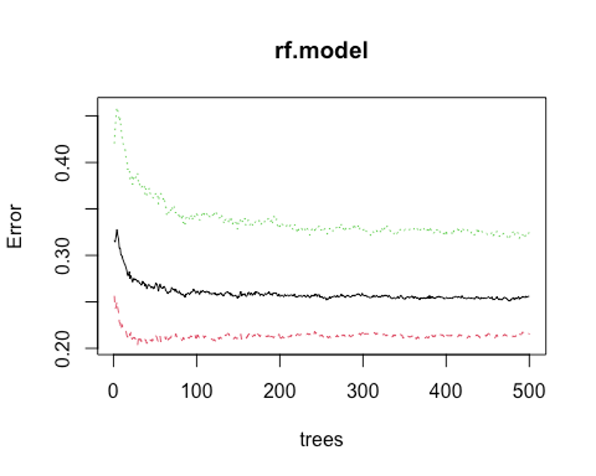
which.min(rf.model$err.rate[, 1])
## [1] 476
모형 정확도를 최적화하기에 필요한 트리수가 476개면 된다는 결과를 얻었다.
- 다시 모형을 만들어 보자.
set.seed(123)
rf.model2 <- randomForest(smoking ~., data = train, ntree = 476)
rf.model2
##
## Call:
##  randomForest(formula = smoking ~ ., data = train, ntree = 476)
##                Type of random forest: classification
##                      Number of trees: 476
## No. of variables tried at each split: 4
##
##         OOB estimate of  error rate: 25.1%
## Confusion matrix:
##       No Yes class.error
## No  1944 523   0.2119984
## Yes  456 977   0.3182135
OOB 오차율이 25.59%에서 25.1%로 약간 떨어졌다.
- test데이터로 어떤 결과가 나오는지 보자.
rf.fit <- predict(rf.model2, newdata = test, type = 'class')
head(rf.fit)
##  28  35 117 126 188 197
## Yes Yes Yes Yes Yes Yes
## Levels: No Yes
rf.confusion <- confusionMatrix(rf.fit, test$smoking, positive = 'Yes')
rf.confusion
## Confusion Matrix and Statistics
##
##           Reference
## Prediction  No Yes
##        No  845 193
##        Yes 212 420
##
##                Accuracy : 0.7575
##                  95% CI : (0.7362, 0.7779)
##     No Information Rate : 0.6329
##     P-Value [Acc > NIR] : <2e-16
##
##                   Kappa : 0.4815
##
##  Mcnemar's Test P-Value : 0.3711
##
##             Sensitivity : 0.6852
##             Specificity : 0.7994
##          Pos Pred Value : 0.6646
##          Neg Pred Value : 0.8141
##              Prevalence : 0.3671
##          Detection Rate : 0.2515
##    Detection Prevalence : 0.3784
##       Balanced Accuracy : 0.7423
##
##        'Positive' Class : Yes
##
rf.confusion$byClass
##          Sensitivity          Specificity       Pos Pred Value
##            0.6851550            0.7994324            0.6645570
##       Neg Pred Value            Precision               Recall
##            0.8140655            0.6645570            0.6851550
##                   F1           Prevalence       Detection Rate
##            0.6746988            0.3670659            0.2514970
## Detection Prevalence    Balanced Accuracy
##            0.3784431            0.7422937
Accuracy : 0.758, Kappa : 0.483, F1 score : 0.676이다.
- 성능을 좀 더 높여보자.
rf_mtry <- seq(4, ncol(train) * 0.8, by = 2)
rf_nodesize <- seq(3, 8, by = 2)
rf_sample_size <- nrow(train) * c(0.7, 0.8)
rf_hyper_grid <- expand.grid(mtry = rf_mtry,
                             nodesize = rf_nodesize,
samplesize = rf_sample_size)- 설정된 파라미터를 바탕으로 모형을 적합한다.
rf_oob_err <- c()

for(i in 1:nrow(rf_hyper_grid)) {

  model <- randomForest(formula = smoking ~.,
                        data = train,
                        mtry = rf_hyper_grid$mtry[i],
                        nodesize = rf_hyper_grid$nodesize[i],
                        samplesize = rf_hyper_grid$samplesize[i])

  rf_oob_err[i] <- model$err.rate[nrow(model$err.rate), 'OOB']
}- 최적의 하이퍼 파라미터를 보자.
rf_hyper_grid[which.min(rf_oob_err), ]
##   mtry nodesize samplesize
## 6 4 5 2730- 위의 파라미터를 토대로 모형을 만들자.
rf_best_model <- randomForest(formula = smoking ~.,
                              data = train,
                              mtry = 4,
                              nodesize = 5,
                              sampsize = 2730,
                              proximity = TRUE,
importance = TRUE)- 변수 중요도를 보자.
varImpPlot(rf_best_model, type = 1)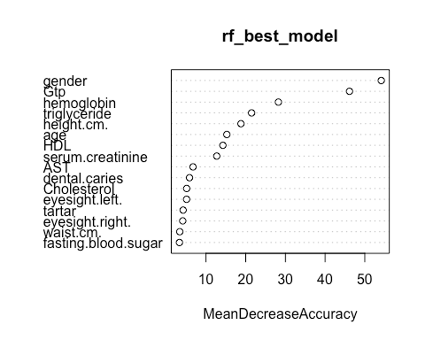
varImpPlot(rf_best_model, type = 2)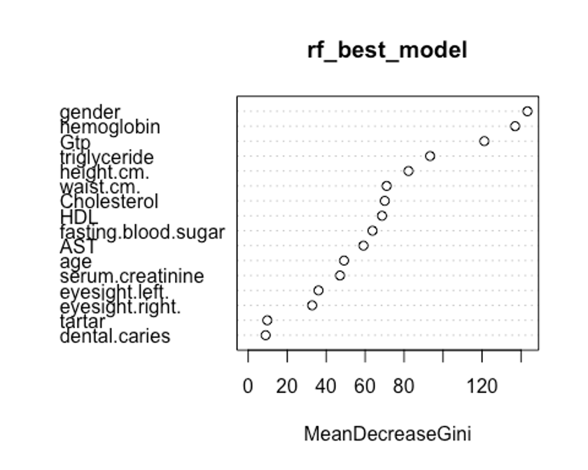
첫번째 plot을 보자. 변수의 값을 랜덤하게 섞었다면, 모델의 정확도가 감소하는 정도를 측정한다.(type = 1)
변수를 랜덤하게 섞는다는 것은 해당 변수가 예측에 미치는 모든 영향력을 제거하는 것을 의미한다. 정확도는 OOB데이터로부터 얻는다. 이는 결국 교차 타당성과 같은 효과를 얻는다.
두번째 plot을 보자. 특정 변수를 기준으로 분할이 일어난 모든 노드에서 불순도 점수의 평균 감소량을 측정한다.(type = 2)
이 지표는 해당 변수가 노드의 불순도를 개선하는데 얼마나 기여했는지를 나타낸다.
그러나 이 지표는 학습데이터를 기반으로 측정되기 때문에 OOB데이터를 가지고 계산한 것에 비해 믿을만하지 못하다.
우리의 plot에서 첫번째와 두번째 plot의 변수 중요도 순서가 다소 다른것을 볼 수 있는데, OOB데이터로부터 정확도 감소량을 측정한 첫번째 plot이 더 믿을만하다.
- predict함수로 예측을 해보자.
rf.fit <- predict(rf_best_model, newdata = test, type = 'class')
rf.best.confusion <- confusionMatrix(rf.fit, test$smoking, positive = 'Yes')
rf.best.confusion
## Confusion Matrix and Statistics
##
##           Reference
## Prediction  No Yes
##        No  842 198
##        Yes 215 415
##
##                Accuracy : 0.7527
##                  95% CI : (0.7313, 0.7732)
##     No Information Rate : 0.6329
##     P-Value [Acc > NIR] : <2e-16
##
##                   Kappa : 0.4708
##
##  Mcnemar's Test P-Value : 0.4311
##
##             Sensitivity : 0.6770
##             Specificity : 0.7966
##          Pos Pred Value : 0.6587
##          Neg Pred Value : 0.8096
##              Prevalence : 0.3671
##          Detection Rate : 0.2485
##    Detection Prevalence : 0.3772
##       Balanced Accuracy : 0.7368
##
##        'Positive' Class : Yes
##
rf.best.confusion$byClass
##          Sensitivity          Specificity       Pos Pred Value
##            0.6769984            0.7965941            0.6587302
##       Neg Pred Value            Precision               Recall
##            0.8096154            0.6587302            0.6769984
##                   F1           Prevalence       Detection Rate
##            0.6677393            0.3670659            0.2485030
## Detection Prevalence    Balanced Accuracy
##            0.3772455            0.7367963
위에서 본 랜덤포레스트 기본 모형(Accuracy : 0.758, Kappa : 0.483, F1 score : 0.676)보다 Accuracy : 0.753, Kappa : 0.471, F1 score : 0.668로 오히려 성능이 떨어졌다.
- ROC커브를 그려보자.
plot(perf.earth, col = 1)
plot(perf.knn, col = 2, add = TRUE)
plot(perf.svm, col = 3, add = TRUE)

rf.pred <- predict(rf_best_model, newdata = test, type = 'prob')
head(rf.pred)
##        No   Yes
## 28  0.438 0.562
## 35  0.288 0.712
## 117 0.280 0.720
## 126 0.440 0.560
## 188 0.274 0.726
## 197 0.410 0.590
rf.pred.yes <- rf.pred[, 2]
head(rf.pred.yes)
##    28    35   117   126   188   197
## 0.562 0.712 0.720 0.560 0.726 0.590
pred.rf <- prediction(rf.pred.yes, test$smoking)
perf.rf <- performance(pred.rf, 'tpr', 'fpr')

plot(perf.rf, col = 4, add = TRUE)
legend(0.6, 0.6, c('MARS', 'KNN', 'SVM', 'RF'), 1:4)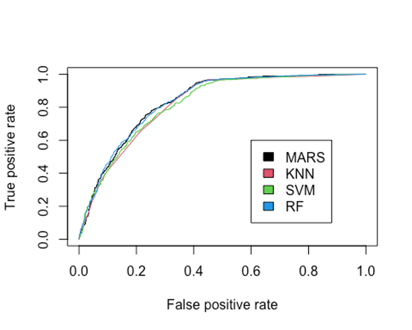
- AUC도 알아보자.
performance(pred.earth, 'auc')@y.values
## [[1]]
## [1] 0.8359002
performance(pred.knn, 'auc')@y.values
## [[1]]
## [1] 0.8207136
performance(pred.svm, 'auc')@y.values
## [[1]]
## [1] 0.82103
performance(pred.rf, 'auc')@y.values
## [[1]]
## [1] 0.8359581
AUC를 분류 성능의 기준으로 삼는다면 랜덤포레스트 모형이 현재까지는 가장 높은 AUC를 보이고 있다(그러나 MARS모형과 거의 유사한 성능이다).
XGBoost
- XGBoost를 사용해서 분석을 해보자.
- scaled_train_dummy, scaled_test_dummy 데이터를 사용한다.
- 그리드를 만들어 보자.
grid <- expand.grid(nrounds = c(75, 150),
                    colsample_bytree = 1,
                    min_child_weight = 1,
                    eta = c(0.01, 0.1, 0.3),
                    gamma = c(0.5, 0.25),
                    subsample = 0.5,
max_depth = c(2, 3))- trainControl인자를 조정힌다. 여기서는 5-fold교차검증을 사용해 보자.
cntrl <- trainControl(method = 'cv',
                      number = 5,
                      verboseIter = TRUE,
                      returnData = FALSE,
returnResamp = 'final')- train()을 사용해 데이터를 학습시킨다.
set.seed(123)
train.xgb <- train(x = scaled_train_dummy[, 1:19],
                   y = scaled_train_dummy[, 20],
                   trControl = cntrl,
                   tuneGrid = grid,
                   method = 'xgbTree')
## + Fold1: eta=0.01, max_depth=2, gamma=0.25, colsample_bytree=1, min_child_weight=1, subsample=0.5, nrounds=150
.
.
.(생략)
## Selecting tuning parameters
## Fitting nrounds = 75, max_depth = 3, eta = 0.1, gamma = 0.5, colsample_bytree = 1, min_child_weight = 1, subsample = 0.5 on full training set
train.xgb
## eXtreme Gradient Boosting
##
## No pre-processing
## Resampling: Cross-Validated (5 fold)
## Summary of sample sizes: 3120, 3121, 3119, 3120, 3120
## Resampling results across tuning parameters:
##
##   eta   max_depth  gamma  nrounds  Accuracy   Kappa
##   0.01  2          0.25    75      0.7361556  0.4537055
##   0.01  2          0.25   150      0.7412848  0.4637720
##   0.01  2          0.50    75      0.7379508  0.4562909
##   0.01  2          0.50   150      0.7423092  0.4658718
##   0.01  3          0.25    75      0.7482069  0.4687925
##   0.01  3          0.25   150      0.7500035  0.4723371
##   0.01  3          0.50    75      0.7433342  0.4562776
##   0.01  3          0.50   150      0.7461537  0.4639333
##   0.10  2          0.25    75      0.7515426  0.4731297
##   0.10  2          0.25   150      0.7510304  0.4713639
##   0.10  2          0.50    75      0.7505143  0.4719341
##   0.10  2          0.50   150      0.7494910  0.4672169
##   0.10  3          0.25    75      0.7500028  0.4684003
##   0.10  3          0.25   150      0.7494906  0.4647166
##   0.10  3          0.50    75      0.7548753  0.4788952
##   0.10  3          0.50   150      0.7538499  0.4753970
##   0.30  2          0.25    75      0.7425643  0.4504028
##   0.30  2          0.25   150      0.7361553  0.4330294
##   0.30  2          0.50    75      0.7530787  0.4705014
##   0.30  2          0.50   150      0.7425603  0.4447263
##   0.30  3          0.25    75      0.7397523  0.4401870
##   0.30  3          0.25   150      0.7353900  0.4285409
##   0.30  3          0.50    75      0.7387178  0.4405370
##   0.30  3          0.50   150      0.7361550  0.4305610
##
## Tuning parameter 'colsample_bytree' was held constant at a value of 1
##
## Tuning parameter 'min_child_weight' was held constant at a value of 1
##
## Tuning parameter 'subsample' was held constant at a value of 0.5
## Accuracy was used to select the optimal model using the largest value.
## The final values used for the model were nrounds = 75, max_depth = 3, eta
##  = 0.1, gamma = 0.5, colsample_bytree = 1, min_child_weight = 1 and subsample
## = 0.5.- 모형을 생성하기 위한 최적 인자들의 조합이 출력되었다.
- xgb.train()에서 사용할 인자 목록을 생성하고, 데이터 프레임을 입력피처의 행렬과 숫자 레이블을 붙인 결과 목록으로 변환한다. 그런 다음, 피처와 식별값을 xgb.DMatrix에서 사용할 입력값으로 변환한다.
param <- list(objective = 'binary:logistic',
              booster = 'gbtree',
              eval_metric = 'error',
              eta = 0.1,
              max_depth = 3,
              subsample = 0.5,
              colsample_bytree = 1,
              gamma = 0.5)
x <- as.matrix(scaled_train_dummy[, 1:19])
y <- ifelse(scaled_train_dummy$smoking == 'Yes', 1, 0)
train.mat <- xgb.DMatrix(data = x, label = y)- 이제 모형을 만들어 보자.
set.seed(123)
xgb.fit <- xgb.train(params = param, data = train.mat, nrounds = 75)- 테스트 세트에 관한 결과를 보기 전에 변수 중요도를 그려 검토해보자.
- 항목은 gain, cover, frequency이렇게 세가지를 검사할 수 있다.
- gain은 피처가 트리에 미치는 정확도의 향상 정도를 나타내는 값, cover는 이 피처와 연관된 전체 관찰값의 상대 수치, frequency는 모든 트리에 관해 피처가 나타난 횟수를 백분율로 나타낸 값이다.
impMatrix <- xgb.importance(feature_names = dimnames(x)[[2]], model = xgb.fit)
impMatrix
##                 Feature        Gain      Cover  Frequency
##  1:            gender.F 0.472958584 0.13350031 0.05432596
##  2:                 Gtp 0.109009315 0.15021325 0.12877264
##  3:        triglyceride 0.058434149 0.08216898 0.09255533
##  4:          hemoglobin 0.058127937 0.09561035 0.09657948
##  5:                 age 0.054295596 0.07963377 0.07243461
##  6:                 AST 0.039614242 0.05136911 0.08853119
##  7:           waist.cm. 0.038446151 0.07838432 0.08450704
##  8:         Cholesterol 0.026314069 0.04533613 0.06639839
##  9:    serum.creatinine 0.025940210 0.04922199 0.05030181
## 10:                 HDL 0.024855993 0.04049101 0.05633803
## 11:          height.cm. 0.023176614 0.05081891 0.04225352
## 12: fasting.blood.sugar 0.021260873 0.04145364 0.06237425
## 13:      eyesight.left. 0.015741720 0.03632828 0.03420523
## 14:            tartar.N 0.014725824 0.02567855 0.03018109
## 15:     eyesight.right. 0.009961228 0.01955187 0.02414487
## 16:     dental.caries.0 0.007137496 0.02023953 0.01609658
xgb.plot.importance(impMatrix, main = 'Gain by Feature')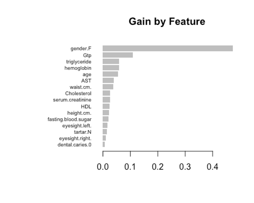
- 다음으로 테스트 세트에 관한 수행 결과를 보자.
library(InformationValue)
##
## Attaching package: 'InformationValue'
## The following object is masked from 'package:genridge':
##
##     precision
## The following objects are masked from 'package:caret':
##
##     confusionMatrix, precision, sensitivity, specificity
pred <- predict(xgb.fit, x)
optimalCutoff(y, pred)
## [1] 0.4784452
testMat <- as.matrix(scaled_test_dummy[, 1:19])
xgb.test <- predict(xgb.fit, testMat)
y.test <- ifelse(scaled_test_dummy$smoking == 'Yes', 1, 0)
confusionMatrix(y.test, xgb.test, threshold = 0.4784452)
##     0   1
## 0 838 200
## 1 219 413
1 - misClassError(y.test, xgb.test, threshold = 0.4784452)
## [1] 0.7491
약 74.91%의 정확도를 보였다.
- F1-score를 계산해보자.
precision <- 413 / (413 + 200)
recall <- 413 / (413 + 219)
f1 <- (2 * precision * recall) / (precision + recall)
f1
## [1] 0.6634538
정확도는 74.91%, F1-score는 0.663으로 랜덤포레스트의 성능보다 살짝 떨어진다.
- ROC커브를 그려보자.
plotROC(y.test, xgb.test)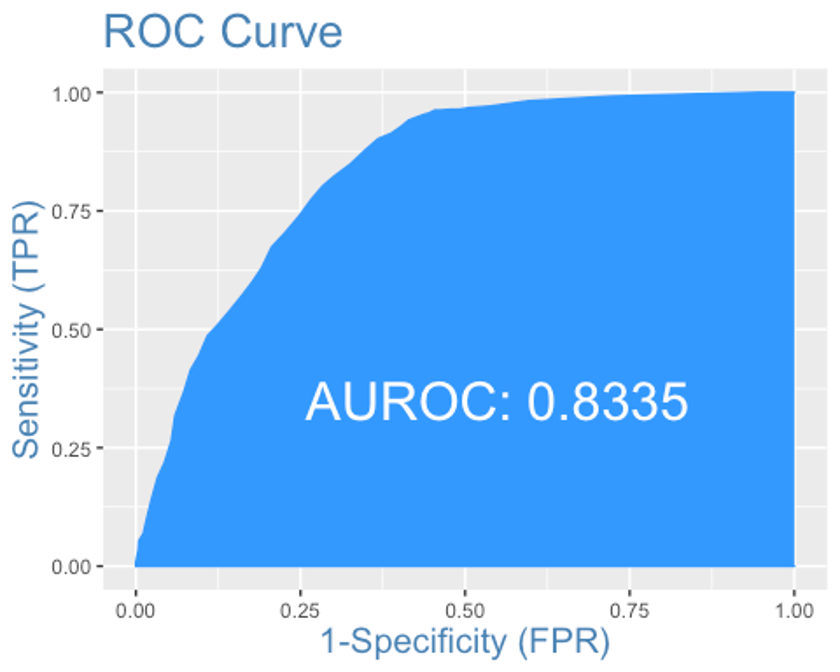
AUC는 0.8335로 MARS모형과 랜덤포레스트 모형보다 약간 떨어진다.
앙상블
- 앙상블 분석을 해보자.
- 데이터는 scaled_train_dummy, scaled_test_dummy를 사용하자.
- 먼저 필요한 패키지를 불러온다.
library(caret)
library(MASS)
library(caretEnsemble)
##
## Attaching package: 'caretEnsemble'
## The following object is masked from 'package:ggplot2':
##
##     autoplot
library(caTools)
library(mlr)
## Loading required package: ParamHelpers
## Warning message: 'mlr' is in 'maintenance-only' mode since July 2019.
## Future development will only happen in 'mlr3'
## (<https://mlr3.mlr-org.com>). Due to the focus on 'mlr3' there might be
## uncaught bugs meanwhile in {mlr} - please consider switching.
##
## Attaching package: 'mlr'
## The following object is masked _by_ '.GlobalEnv':
##
##     f1
## The following object is masked from 'package:e1071':
##
##     impute
## The following object is masked from 'package:ROCR':
##
##     performance
## The following object is masked from 'package:caret':
##
##     train
library(ggplot2)
library(HDclassif)
library(gbm)
## Loaded gbm 2.1.8
library(mboost)
## Loading required package: parallel
## Loading required package: stabs
##
## Attaching package: 'stabs'
## The following object is masked from 'package:mlr':
##
##     subsample
##
## Attaching package: 'mboost'
## The following object is masked from 'package:partykit':
##
##     varimp
## The following objects are masked from 'package:psych':
##
##     %+%, AUC
## The following object is masked from 'package:pastecs':
##
##     extract
## The following object is masked from 'package:ggplot2':
##
## %+%- 5-fold교차검증을 사용하자.
control <- trainControl(method = 'cv', number = 5,
                        savePredictions = 'final',
                        classProbs = TRUE,
summaryFunction = twoClassSummary) - 이제 모형을 학습시키자. 분류트리, MARS, KNN을 사용해보자.
set.seed(123)
models <- caretList(smoking ~., data = scaled_train_dummy,
                    trControl = control,
                    metric = 'ROC',
                    methodList = c('earth', 'svmLinear', 'treebag'))
## Warning in trControlCheck(x = trControl, y = target): indexes not defined in
## trControl. Attempting to set them ourselves, so each model in the ensemble will
## have the same resampling indexes.
## Warning: glm.fit: fitted probabilities numerically 0 or 1 occurred

## Warning: glm.fit: fitted probabilities numerically 0 or 1 occurred

## Warning: glm.fit: fitted probabilities numerically 0 or 1 occurred
models
## $earth
## Multivariate Adaptive Regression Spline
##
## 3900 samples
##   19 predictor
##    2 classes: 'No', 'Yes'
##
## No pre-processing
## Resampling: Cross-Validated (5 fold)
## Summary of sample sizes: 3120, 3120, 3119, 3120, 3121
## Resampling results across tuning parameters:
##
##   nprune  ROC        Sens       Spec
##    2      0.7546569  0.5581649  0.9511489
##   13      0.8266104  0.7802933  0.6860237
##   25      0.8293113  0.7831315  0.6832290
##
## Tuning parameter 'degree' was held constant at a value of 1
## ROC was used to select the optimal model using the largest value.
## The final values used for the model were nprune = 25 and degree = 1.
##
## $svmLinear
## Support Vector Machines with Linear Kernel
##
## 3900 samples
##   19 predictor
##    2 classes: 'No', 'Yes'
##
## No pre-processing
## Resampling: Cross-Validated (5 fold)
## Summary of sample sizes: 3120, 3120, 3119, 3120, 3121
## Resampling results:
##
##   ROC        Sens       Spec
##   0.8159807  0.8025827  0.613428
##
## Tuning parameter 'C' was held constant at a value of 1
##
## $treebag
## Bagged CART
##
## 3900 samples
##   19 predictor
##    2 classes: 'No', 'Yes'
##
## No pre-processing
## Resampling: Cross-Validated (5 fold)
## Summary of sample sizes: 3120, 3120, 3119, 3120, 3121
## Resampling results:
##
##   ROC        Sens       Spec
##   0.8156656  0.7811047  0.6650813
##
##
## attr(,"class")
## [1] "caretList"- 데이터 프레임 안의 테스트 세트에서 ’Yes’값에 관한 예측값을 얻어오자.
model_preds <- lapply(models, predict, newdata = scaled_test_dummy, type = 'prob')
model_preds <- lapply(model_preds, function(x) x[, 'Yes'])
model_preds <- data.frame(model_preds)- stack으로 로지스틱 회귀 모형을 쌓아보자
stack <- caretStack(models, method = 'glm', metric = 'ROC',
                    trControl = trainControl(
                      method = 'boot', number = 5,
                      savePredictions = 'final',
                      classProbs = TRUE,
                      summaryFunction = twoClassSummary
                    ))
summary(stack)
##
## Call:
## NULL
##
## Deviance Residuals:
##     Min       1Q   Median       3Q      Max
## -2.2103  -0.7327  -0.3556   0.8404   2.4086
##
## Coefficients:
##             Estimate Std. Error z value Pr(>|z|)
## (Intercept)   2.7922     0.1160  24.078  < 2e-16 ***
## earth        -2.5350     0.3644  -6.958 3.46e-12 ***
## svmLinear    -1.4454     0.3582  -4.035 5.47e-05 ***
## treebag      -1.7586     0.2900  -6.065 1.32e-09 ***
## ---
## Signif. codes:  0 '***' 0.001 '**' 0.01 '*' 0.05 '.' 0.1 ' ' 1
##
## (Dispersion parameter for binomial family taken to be 1)
##
##     Null deviance: 5129.1  on 3899  degrees of freedom
## Residual deviance: 3724.1  on 3896  degrees of freedom
## AIC: 3732.1
##
## Number of Fisher Scoring iterations: 5
모형의 계수가 모두 유의하다.
- 앙상블에 사용된 학습자의 각 예측결과를 비교해보자.
prob <- 1 - predict(stack, newdata = scaled_test_dummy, type = 'prob')
model_preds$ensemble <- prob
colAUC(model_preds, scaled_test_dummy$smoking)
##                earth svmLinear   treebag  ensemble
## No vs. Yes 0.8327456 0.8209652 0.8140494 0.8366857
각 모형의 AUC를 봤을 때 앙상블 모형이 MARS모형만 사용한 것보다 조금 더 나은 성능을 보인다.
class <- predict(stack, newdata = scaled_test_dummy, type = 'raw')
head(class)
## [1] Yes Yes Yes No  Yes Yes
## Levels: No Yes
detach("package:InformationValue", unload = TRUE)
ensemble.confusion <- confusionMatrix(class, scaled_test_dummy$smoking, positive = 'Yes')
ensemble.confusion
## Confusion Matrix and Statistics
##
##           Reference
## Prediction  No Yes
##        No  865 226
##        Yes 192 387
##
##                Accuracy : 0.7497
##                  95% CI : (0.7282, 0.7703)
##     No Information Rate : 0.6329
##     P-Value [Acc > NIR] : <2e-16
##
##                   Kappa : 0.455
##
##  Mcnemar's Test P-Value : 0.1065
##
##             Sensitivity : 0.6313
##             Specificity : 0.8184
##          Pos Pred Value : 0.6684
##          Neg Pred Value : 0.7929
##              Prevalence : 0.3671
##          Detection Rate : 0.2317
##    Detection Prevalence : 0.3467
##       Balanced Accuracy : 0.7248
##
##        'Positive' Class : Yes
##
ensemble.confusion$byClass
##          Sensitivity          Specificity       Pos Pred Value
##            0.6313214            0.8183538            0.6683938
##       Neg Pred Value            Precision               Recall
##            0.7928506            0.6683938            0.6313214
##                   F1           Prevalence       Detection Rate
##            0.6493289            0.3670659            0.2317365
## Detection Prevalence    Balanced Accuracy
##            0.3467066            0.7248376
Conclusion
- 모든 분석이 끝났다.
- 총 6개의 모형을 만들었고, 각각의 모형의 평가 지표가 어떻게 나왔는지 비교해보자.
| - | MARS | KNN | SVM | RandomForest | XGBoost | Ensemble |
|---|---|---|---|---|---|---|
| Accuracy | 0.761 | 0.745 | 0.645 | 0.753 | 0.749 | 0.750 |
| F1-score | 0.690 | 0.668 | 0.505 | 0.471 | 0.663 | 0.649 |
| Kappa | 0.496 | 0.461 | 0.228 | 0.668 | - | 0.455 |
| AUC | 0.836 | 0.821 | 0.821 | 0.836 | 0.834 | 0.837 |
그렇다면 위 6개의 모형 중 어떤 모형을 선택해야 하는가?
우선 6개의 모형 중 SVM이 가장 좋지 않은 성능을 보이고 있다. 다른 모형에 비해서 F1-score와 Kappa 통계량이 눈에 띄게 낮은 수치를 보인다. Accuracy도 가장 낮은 수치를 보여 오분류율이 높은 것으로 판단된다.
그 다음으로 랜덤포레스트 모델을 보면 Accuracy는 다른 모델들과 비슷한 수준이나 F1-score가 유독 낮은데 이는 recall이 다른 모형에 비해 낮기 때문인 것으로 보인다.
그 외 나머지 모델들(MARS, KNN, XGBoost, Ensemble)은 거의 비슷한 분류 성능을 보이는데 하나의 모형을 골라야 한다면 MARS모형을 선택하겠다.
MARS는 데이터 전처리 과정이 다른 모델에 비해서 중요하지 않은 편이고, 변수를 자동으로 선택해 어느 변수가 중요한 변수인지 쉽게 알 수 있다.
또한 상호작용항을 지원하며, 다양한 그래프를 통한 이해와 설명이 간편해 이해관계자를 이해시키기 쉽다는 장점이 있다.
사용한 패키지
caret, pastecs, psych, PerformanceAnalytics, Fselector, GGally, gridExtra, gapminder, dplyr, class, kknn, e1071, MASS, reshape2, ggplot2, kernlab, corrplot, rpart, partykit, genridge, randomForest, xgboost, Boruta, caretEnsemble, caTools, mlr, HDclassif, earth, Formula, plotmo, plotrix, ROCR, InformationValue, gbm, mboost