South German Credit Data Set
데이터 출처
The widely used Statlog German credit data, as of November 2019, suffers from severe errors in the coding information and does not come with any background information. The 'South German Credit' data provide a correction and some background information, based on the Open Data LMU (2010) representation of the same data and several other German language resources.
데이터는 총 21개의 칼럼과 1000개의 rows로 구성
| Header | Description |
|---|---|
| status | status of the debtor's checking account with the bank (categorical) |
| duration | credit duration in months (quantitative) |
| credit_history | history of compliance with previous or concurrent credit contracts (categorical) |
| purpose | purpose for which the credit is needed (categorical) |
| amount | credit amount in DM (quantitative) |
| savings | debtor's savings (categorical) |
| employment_duration | duration of debtor's employment with current employer |
| installment_rate | credit installments as a percentage of debtor's disposable income |
| personal_status_sex | combined information on sex and marital status (categorical) |
| other_debtors | Is there another debtor or a guarantor for the credit? (categorical) |
| present_residence | length of time (in years) the debtor lives in the present residence |
| property | the debtor's most valuable property |
| age | age in years (quantitative) |
| other_installment_plans | installment plans from providers other than the credit-giving bank (categorical) |
| housing | type of housing the debtor lives in (categorical) |
| number_credits | number of credits including the current one the debtor has (or had) at this bank |
| job | quality of debtor's job (ordinal) |
| people_liable | number of persons who financially depend on the debtor |
| telephone | Is there a telephone landline registered on the debtor's name? (binary; remember that the data are from the 1970s) |
| foreign_worker | Is the debtor a foreign worker? (binary) |
| credit_risk | Has the credit contract been complied with (good) or not (bad) ? (binary) |
EDA
- 데이터를 불러오고, 독일어로 되어있는 변수명을 알아보기 쉽게 영어로 바꿔주자.
dat <- read.table("SouthGermanCredit.asc", header=TRUE)
nam_fahrmeirbook <- colnames(dat)
nam_evtree <- c("status", "duration", "credit_history", "purpose", "amount",
                "savings", "employment_duration", "installment_rate",
                "personal_status_sex", "other_debtors",
                "present_residence", "property",
                "age", "other_installment_plans",
                "housing", "number_credits",
                "job", "people_liable", "telephone", "foreign_worker",
                "credit_risk")
names(dat) <- nam_evtree
for (i in setdiff(1:21, c(2,4,5,13)))
  dat[[i]] <- factor(dat[[i]])
dat[[4]] <- factor(dat[[4]], levels=as.character(0:10))
levels(dat$credit_risk) <- c("bad", "good")
levels(dat$status) = c("no checking account",
                         "... < 0 DM",
                         "0<= ... < 200 DM",
                         "... >= 200 DM / salary for at least 1 year")
levels(dat$credit_history) <- c(
  "delay in paying off in the past",
  "critical account/other credits elsewhere",
  "no credits taken/all credits paid back duly",
  "existing credits paid back duly till now",
  "all credits at this bank paid back duly")
levels(dat$purpose) <- c(
  "others",
  "car (new)",
  "car (used)",
  "furniture/equipment",
  "radio/television",
  "domestic appliances",
  "repairs",
  "education",
  "vacation",
  "retraining",
  "business")
levels(dat$savings) <- c("unknown/no savings account",
                         "... <  100 DM",
                         "100 <= ... <  500 DM",
                         "500 <= ... < 1000 DM",
                         "... >= 1000 DM")
levels(dat$employment_duration) <-
                  c(  "unemployed",
                      "< 1 yr",
                      "1 <= ... < 4 yrs",
                      "4 <= ... < 7 yrs",
                      ">= 7 yrs")
dat$installment_rate <- ordered(dat$installment_rate)
levels(dat$installment_rate) <- c(">= 35",
                                  "25 <= ... < 35",
                                  "20 <= ... < 25",
                                  "< 20")
levels(dat$other_debtors) <- c(
  "none",
  "co-applicant",
  "guarantor"
)
levels(dat$personal_status_sex) <- c(
  "male : divorced/separated",
  "female : non-single or male : single",
  "male : married/widowed",
  "female : single")
dat$present_residence <- ordered(dat$present_residence)
levels(dat$present_residence) <- c("< 1 yr",
                                   "1 <= ... < 4 yrs",
                                   "4 <= ... < 7 yrs",
                                   ">= 7 yrs")
levels(dat$property) <- c(
  "unknown / no property",
  "car or other",
  "building soc. savings agr./life insurance",
  "real estate"
)
levels(dat$other_installment_plans) <- c(
  "bank",
  "stores",
  "none"
)
levels(dat$housing) <- c("for free", "rent", "own")
dat$number_credits <- ordered(dat$number_credits)
levels(dat$number_credits) <- c("1", "2-3", "4-5", ">= 6")
levels(dat$job) <- c(
  "unemployed/unskilled - non-resident",
  "unskilled - resident",
  "skilled employee/official",
  "manager/self-empl./highly qualif. employee"
)
levels(dat$people_liable) <- c("3 or more", "0 to 2")
levels(dat$telephone) <- c("no", "yes (under customer name)")
levels(dat$foreign_worker) <- c("yes", "no")- 데이터를 테이블 형식에서 데이터 프레임 형식으로 바꾸고 데이터를 기본 구조를 파악해보자.
df <- as.data.frame(dat)
dim(df)
## [1] 1000   21
str(df)
## 'data.frame':    1000 obs. of  21 variables:
##  $ status                 : Factor w/ 4 levels "no checking account",..: 1 1 2 1 1 1 1 1 4 2 ...
##  $ duration               : int  18 9 12 12 12 10 8 6 18 24 ...
##  $ credit_history         : Factor w/ 5 levels "delay in paying off in the past",..: 5 5 3 5 5 5 5 5 5 3 ...
##  $ purpose                : Factor w/ 11 levels "others","car (new)",..: 3 1 10 1 1 1 1 1 4 4 ...
##  $ amount                 : int  1049 2799 841 2122 2171 2241 3398 1361 1098 3758 ...
##  $ savings                : Factor w/ 5 levels "unknown/no savings account",..: 1 1 2 1 1 1 1 1 1 3 ...
##  $ employment_duration    : Factor w/ 5 levels "unemployed","< 1 yr",..: 2 3 4 3 3 2 4 2 1 1 ...
##  $ installment_rate       : Ord.factor w/ 4 levels ">= 35"<"25 <= ... < 35"<..: 4 2 2 3 4 1 1 2 4 1 ...
##  $ personal_status_sex    : Factor w/ 4 levels "male : divorced/separated",..: 2 3 2 3 3 3 3 3 2 2 ...
##  $ other_debtors          : Factor w/ 3 levels "none","co-applicant",..: 1 1 1 1 1 1 1 1 1 1 ...
##  $ present_residence      : Ord.factor w/ 4 levels "< 1 yr"<"1 <= ... < 4 yrs"<..: 4 2 4 2 4 3 4 4 4 4 ...
##  $ property               : Factor w/ 4 levels "unknown / no property",..: 2 1 1 1 2 1 1 1 3 4 ...
##  $ age                    : int  21 36 23 39 38 48 39 40 65 23 ...
##  $ other_installment_plans: Factor w/ 3 levels "bank","stores",..: 3 3 3 3 1 3 3 3 3 3 ...
##  $ housing                : Factor w/ 3 levels "for free","rent",..: 1 1 1 1 2 1 2 2 2 1 ...
##  $ number_credits         : Ord.factor w/ 4 levels "1"<"2-3"<"4-5"<..: 1 2 1 2 2 2 2 1 2 1 ...
##  $ job                    : Factor w/ 4 levels "unemployed/unskilled - non-resident",..: 3 3 2 2 2 2 2 2 1 1 ...
##  $ people_liable          : Factor w/ 2 levels "3 or more","0 to 2": 2 1 2 1 2 1 2 1 2 2 ...
##  $ telephone              : Factor w/ 2 levels "no","yes (under customer name)": 1 1 1 1 1 1 1 1 1 1 ...
##  $ foreign_worker         : Factor w/ 2 levels "yes","no": 2 2 2 1 1 1 1 1 2 2 ...
##  $ credit_risk            : Factor w/ 2 levels "bad","good": 2 2 2 2 2 2 2 2 2 2 ...
summary(df)
##                                         status       duration
##  no checking account                       :274   Min.   : 4.0
##  ... < 0 DM                                :269   1st Qu.:12.0
##  0<= ... < 200 DM                          : 63   Median :18.0
##  ... >= 200 DM / salary for at least 1 year:394   Mean   :20.9
##                                                   3rd Qu.:24.0
##                                                   Max.   :72.0
##
##                                      credit_history                purpose
##  delay in paying off in the past            : 40    furniture/equipment:280
##  critical account/other credits elsewhere   : 49    others             :234
##  no credits taken/all credits paid back duly:530    car (used)         :181
##  existing credits paid back duly till now   : 88    car (new)          :103
##  all credits at this bank paid back duly    :293    retraining         : 97
##                                                     repairs            : 50
##                                                     (Other)            : 55
##      amount                            savings          employment_duration
##  Min.   :  250   unknown/no savings account:603   unemployed      : 62
##  1st Qu.: 1366   ... <  100 DM             :103   < 1 yr          :172
##  Median : 2320   100 <= ... <  500 DM      : 63   1 <= ... < 4 yrs:339
##  Mean   : 3271   500 <= ... < 1000 DM      : 48   4 <= ... < 7 yrs:174
##  3rd Qu.: 3972   ... >= 1000 DM            :183   >= 7 yrs        :253
##  Max.   :18424
##
##        installment_rate                           personal_status_sex
##  >= 35         :136     male : divorced/separated           : 50
##  25 <= ... < 35:231     female : non-single or male : single:310
##  20 <= ... < 25:157     male : married/widowed              :548
##  < 20          :476     female : single                     : 92
##
##
##
##       other_debtors        present_residence
##  none        :907   < 1 yr          :130
##  co-applicant: 41   1 <= ... < 4 yrs:308
##  guarantor   : 52   4 <= ... < 7 yrs:149
##                     >= 7 yrs        :413
##
##
##
##                                       property        age
##  unknown / no property                    :282   Min.   :19.00
##  car or other                             :232   1st Qu.:27.00
##  building soc. savings agr./life insurance:332   Median :33.00
##  real estate                              :154   Mean   :35.54
##                                                  3rd Qu.:42.00
##                                                  Max.   :75.00
##
##  other_installment_plans     housing    number_credits
##  bank  :139              for free:179   1   :633
##  stores: 47              rent    :714   2-3 :333
##  none  :814              own     :107   4-5 : 28
##                                         >= 6:  6
##
##
##
##                                          job        people_liable
##  unemployed/unskilled - non-resident       : 22   3 or more:155
##  unskilled - resident                      :200   0 to 2   :845
##  skilled employee/official                 :630
##  manager/self-empl./highly qualif. employee:148
##
##
##
##                      telephone   foreign_worker credit_risk
##  no                       :596   yes: 37        bad :300
##  yes (under customer name):404   no :963        good:700
##
##
##
##
##
sum(is.na(df))
## [1] 0
21개의 피처중 3개만 연속형 피처이고 나머지는 factor형이다. 결측치는 없다.
- 먼저 필요한 패키지들을 먼저 불러오자.
library(DMwR2)
## Registered S3 method overwritten by 'quantmod':
##   method            from
##   as.zoo.data.frame zoo
library(pastecs)
library(psych)
library(caret)
## Loading required package: ggplot2
##
## Attaching package: 'ggplot2'
## The following objects are masked from 'package:psych':
##
##     %+%, alpha
## Loading required package: lattice
library(ggplot2)
library(GGally)
## Registered S3 method overwritten by 'GGally':
##   method from
##   +.gg   ggplot2
library(smotefamily)
library(naniar)
library(reshape2)
library(gridExtra)
library(gapminder)
library(dplyr)
##
## Attaching package: 'dplyr'
## The following object is masked from 'package:gridExtra':
##
##     combine
## The following objects are masked from 'package:pastecs':
##
##     first, last
## The following objects are masked from 'package:stats':
##
##     filter, lag
## The following objects are masked from 'package:base':
##
##     intersect, setdiff, setequal, union
library(PerformanceAnalytics)
## Loading required package: xts
## Loading required package: zoo
##
## Attaching package: 'zoo'
## The following objects are masked from 'package:base':
##
##     as.Date, as.Date.numeric
##
## Attaching package: 'xts'
## The following objects are masked from 'package:dplyr':
##
##     first, last
## The following objects are masked from 'package:pastecs':
##
##     first, last
##
## Attaching package: 'PerformanceAnalytics'
## The following object is masked from 'package:graphics':
##
##     legend
library(FSelector)
library(Boruta)
library(ROSE)
## Loaded ROSE 0.0-4- 탐색적 분석으로 첨도와 왜도를 확인해보자.
describeBy(df[, c(2, 5, 13)], df$credit_risk, mat = FALSE)
##
##  Descriptive statistics by group
## group: bad
##          vars   n    mean      sd median trimmed     mad min   max range skew
## duration    1 300   24.86   13.28   24.0   23.59   17.79   6    72    66 0.83
## amount      2 300 3938.13 3535.82 2574.5 3291.18 2092.69 433 18424 17991 1.57
## age         3 300   33.96   11.23   31.0   32.37    9.64  19    74    55 1.14
##          kurtosis     se
## duration     0.03   0.77
## amount       2.05 204.14
## age          0.73   0.65
## ------------------------------------------------------------
## group: good
##          vars   n    mean      sd median trimmed     mad min   max range skew
## duration    1 700   19.21   11.08     18   17.88    8.90   4    60    56 1.18
## amount      2 700 2985.44 2401.50   2244 2564.21 1485.57 250 15857 15607 1.94
## age         3 700   36.22   11.35     34   34.92   10.38  19    75    56 0.98
##          kurtosis    se
## duration     1.38  0.42
## amount       4.62 90.77
## age          0.59  0.43
결과변수인 ’credit_risk’에서 bad그룹의 duration의 평균보다 good그룹의 평균이 약 5개월 정도 낮은것으로 나타났고, amount의 평균은 bad그룹이 good그룹보다 약 1000DM많은 것으로 나타났다. (즉 신용 계약을 준수한 그룹(good)이 계약을 준수하지 않은 그룹(bad)보다 더 작은 돈을 빌렸다.)
또한 나이의 평균은 bad그룹이 33.9, good그룹이 36.2세로 두 그룹의 차가 2.3으로 큰 차이는 아닌 것으로 보인다.
’age’변수의 왜도와 첨도는 bad그룹과 good그룹이 거의 차이나지 않지만, ’duration’과 ’amount’변수의 왜도와 첨도는 bad그룹보다 good그룹이 조금씩 더 크다.
따라서 bad그룹보다 good그룹의 ‘duration’과 ’amount’ 변수의 데이터가 조금 더 왼쪽에 쏠려있고 약간 더 뾰족한 분포를 보일것으로 예측된다.
- 변수별 분포를 그래프를 그려 확인해보자.
- 먼저 수치형 변수부터 보자.
ggpairs(df, columns = c(2, 5, 13), aes(colour = credit_risk, alpha = 0.4))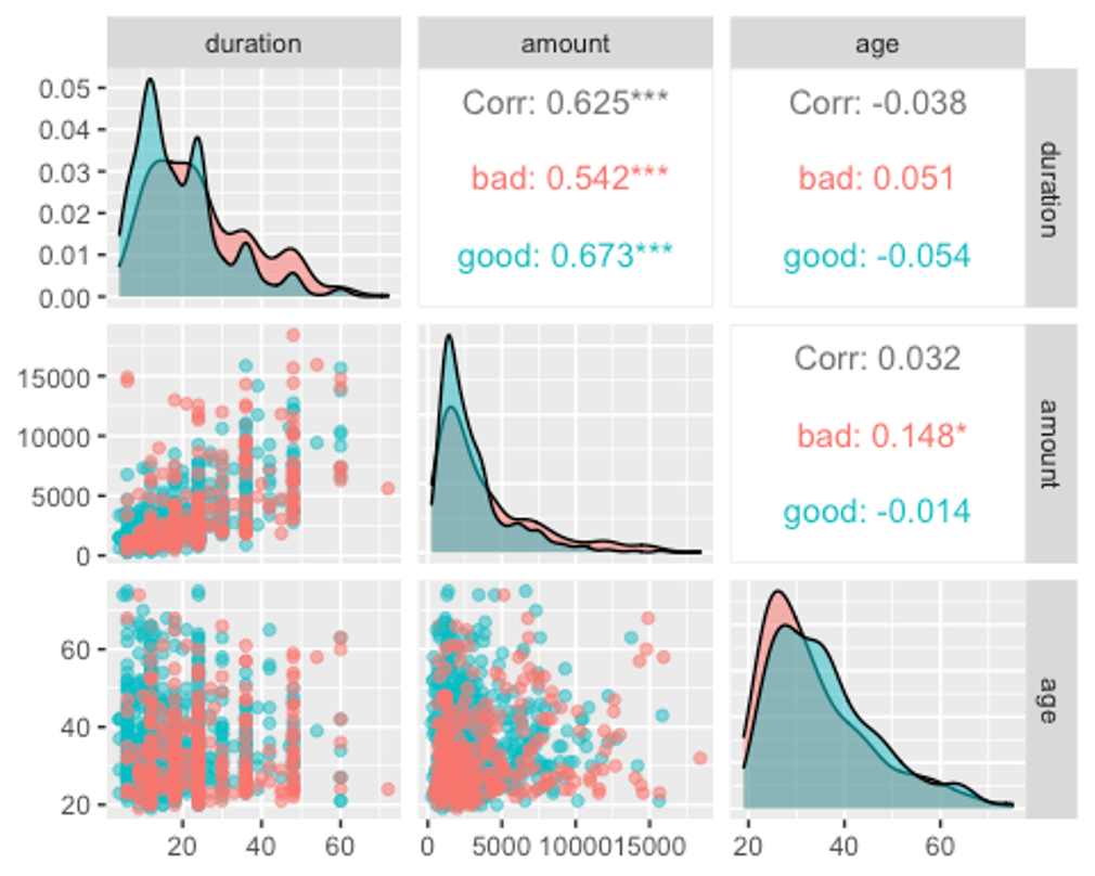
위에서 첨도와 왜도분석에서 보았듯이 ‘duration’과 ’amount’ 변수는 bad그룹보다 good그룹이 더 왼쪽으로 쏠리고 더 뾰족한 분포를 보인다.
반대로 ’age’변수는 good그룹보다 bad그룹이 더 왼쪽으로 쏠리고 살짝 더 뾰족한 분포를 보이고 있다.
또한 ‘duration’과 ’amount’ 변수간의 상관관계가 0.625로 살짝 높은편이다.
- 다음으로 factor형 변수가 어떤 분포를 보이고 있는지 보자.
- factor형 변수가 결과변수를 제외하고 총 17개로 많으므로 두번에 걸쳐서 나눠 보자.
ggpairs(df, columns = c(1, 3, 4, 6, 7, 8, 9, 10), aes(colour = credit_risk, alpha = 0.4))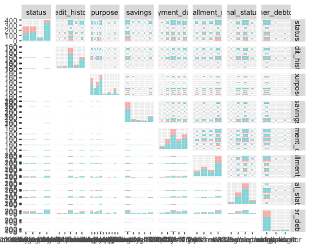
왼쪽 위부터 오른쪽 아래로 가는 대각선에 위치하는 그래프를 보면 된다.
’status’변수는 채무자의 은행 당좌 예금 상태를 나타내는데 200DM이상이 가장 많았고 0이상 200DM미만이 가장 작다.
여기서 ’other_debtors’가 가장 분포의 차이가 두드러지는데 none이 907개, co-applicant가 41개, guarantor가 52개의 데이터로 카테고리별 차이가 10배 이상으로 크다.
- 나머지 factor형 변수들의 분포도 보자.
ggpairs(df, columns = c(11, 12, 14, 15, 16, 17, 18, 19, 20), aes(colour = credit_risk, alpha = 0.4))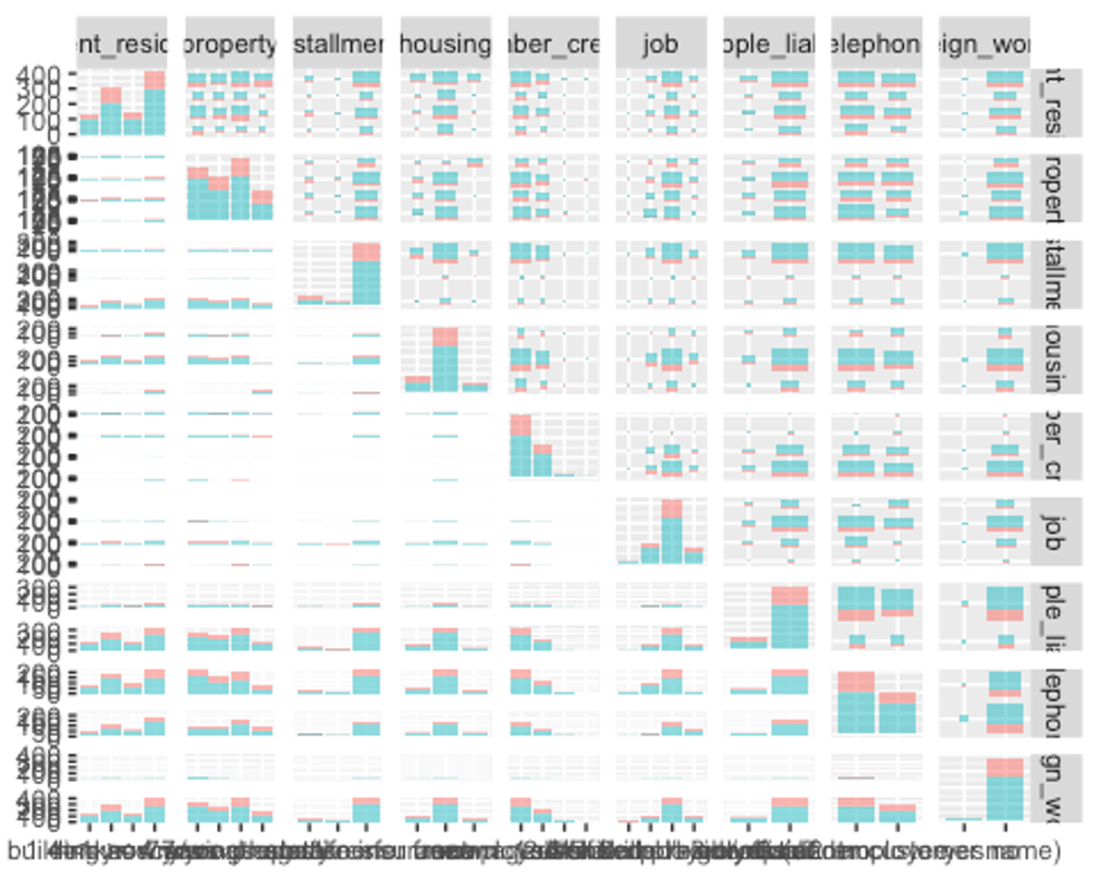
여기서 특이한 변수는 ’other_installment_plans’로 보이는데, 신용 대출 은행 이외의 제공자로부터 받은 할부금이 대부분 없는것(none)으로 나타났다.
또한 ’foreign_worker’변수를 보면 은행에서 돈을 빌린 대부분의 사람이 외국인이 아닌 내국인인 것으로 나타났다.
- 이제 수치형 변수에 이상치가 있는지 확인해보자.
- 데이터의 범위가 변수별로 차이나므로 평균이0, 분산이 1이 되도록 스케일링 하고 데이터를 wide형식에서 long형식으로 바꿔주자.
df_numeric <- df[, c(2, 5, 13, 21)]
model_scale <- preProcess(df_numeric, method = c('center', 'scale'))
scaled_df <- predict(model_scale, df_numeric)
melt_df <- melt(scaled_df, id.vars = 'credit_risk')
head(melt_df)
##   credit_risk variable      value
## 1        good duration -0.2407368
## 2        good duration -0.9870788
## 3        good duration -0.7382981
## 4        good duration -0.7382981
## 5        good duration -0.7382981
## 6        good duration -0.9041519
p1 <- ggplot(melt_df, aes(x = variable, y = value, fill = credit_risk)) + geom_boxplot()
p1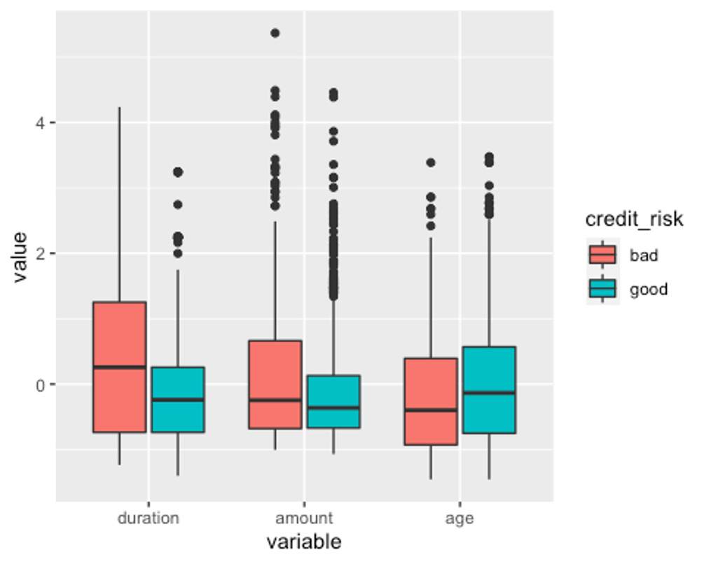
수치형 변수인 duration과 amount, age에 모두 이상치가 있는 것으로 나타났다.
하지만 여기서 이상치로 찍힌 점들은 제 1사분위수 - (1.5IQR)보다 작거나 제3사분위수 + (1.5IQR)보다 큰 수인데, 모든 상황에서 이 수치보다 크거나 작다고 이상치라고 할 수 없다.
현재 age데이터의 최솟값은 19, 최댓값은 75인데 이를 이상치라고 볼 수 없다.
duraion과 amount의 최댓값은 각각 72와 18424인데 이를 명확하게 이상치라고 볼 근거가 없으므로 사분위수 99%범위 밖의 이상치만 75% 사분위수로 바꿔주겠다.
dura_99 <- quantile(df$duration, 0.99)
dura_75 <- quantile(df$duration, 0.75)
amount_99 <- quantile(df$amount, 0.99)
amount_75 <- quantile(df$amount, 0.75)
df$duration <- ifelse(df$duration > dura_99, dura_75, df$duration)
df$amount <- ifelse(df$amount > amount_99, amount_75, df$amount)- 이상치 변경 후의 boxplot을 그려보자.
df_numeric2 <- df[, c(2, 5, 13, 21)]
model_scale2 <- preProcess(df_numeric2, method = c('center', 'scale'))
scaled_df2 <- predict(model_scale2, df_numeric2)
melt_df2 <- melt(scaled_df2, id.vars = 'credit_risk')
head(melt_df2)
##   credit_risk variable      value
## 1        good duration -0.2389069
## 2        good duration -0.9920284
## 3        good duration -0.7409879
## 4        good duration -0.7409879
## 5        good duration -0.7409879
## 6        good duration -0.9083482
p1 <- ggplot(melt_df2, aes(x = variable, y = value, fill = credit_risk)) + geom_boxplot()
p1
잘 변경된 것으로 보인다.
- 다음으로 분산이 0에 가까운 변수를 제거하자.
nearZeroVar(df, saveMetrics = TRUE)
##                         freqRatio percentUnique zeroVar   nzv
## status                   1.437956           0.4   FALSE FALSE
## duration                 1.033520           3.2   FALSE FALSE
## credit_history           1.808874           0.5   FALSE FALSE
## purpose                  1.196581           1.0   FALSE FALSE
## amount                   3.333333          91.4   FALSE FALSE
## savings                  3.295082           0.5   FALSE FALSE
## employment_duration      1.339921           0.5   FALSE FALSE
## installment_rate         2.060606           0.4   FALSE FALSE
## personal_status_sex      1.767742           0.4   FALSE FALSE
## other_debtors           17.442308           0.3   FALSE FALSE
## present_residence        1.340909           0.4   FALSE FALSE
## property                 1.177305           0.4   FALSE FALSE
## age                      1.020408           5.3   FALSE FALSE
## other_installment_plans  5.856115           0.3   FALSE FALSE
## housing                  3.988827           0.3   FALSE FALSE
## number_credits           1.900901           0.4   FALSE FALSE
## job                      3.150000           0.4   FALSE FALSE
## people_liable            5.451613           0.2   FALSE FALSE
## telephone                1.475248           0.2   FALSE FALSE
## foreign_worker          26.027027           0.2   FALSE  TRUE
## credit_risk              2.333333           0.2   FALSE FALSE
table(df$foreign_worker)
##
## yes  no
##  37 963
’foreign_worker’변수의 분산이 0에 가까운것으로 나타났다. 위의 그래프에서 보았다싶이 카테고리에서 외국인의 수는 37, 내국인의 수는 963으로 차이가 많이나 모델링에 유용하지 않다.
- ’foreign_worker’변수를 제거하자.
df2 <- df[, -nearZeroVar(df)]
str(df2)
## 'data.frame':    1000 obs. of  20 variables:
##  $ status                 : Factor w/ 4 levels "no checking account",..: 1 1 2 1 1 1 1 1 4 2 ...
##  $ duration               : num  18 9 12 12 12 10 8 6 18 24 ...
##  $ credit_history         : Factor w/ 5 levels "delay in paying off in the past",..: 5 5 3 5 5 5 5 5 5 3 ...
##  $ purpose                : Factor w/ 11 levels "others","car (new)",..: 3 1 10 1 1 1 1 1 4 4 ...
##  $ amount                 : num  1049 2799 841 2122 2171 ...
##  $ savings                : Factor w/ 5 levels "unknown/no savings account",..: 1 1 2 1 1 1 1 1 1 3 ...
##  $ employment_duration    : Factor w/ 5 levels "unemployed","< 1 yr",..: 2 3 4 3 3 2 4 2 1 1 ...
##  $ installment_rate       : Ord.factor w/ 4 levels ">= 35"<"25 <= ... < 35"<..: 4 2 2 3 4 1 1 2 4 1 ...
##  $ personal_status_sex    : Factor w/ 4 levels "male : divorced/separated",..: 2 3 2 3 3 3 3 3 2 2 ...
##  $ other_debtors          : Factor w/ 3 levels "none","co-applicant",..: 1 1 1 1 1 1 1 1 1 1 ...
##  $ present_residence      : Ord.factor w/ 4 levels "< 1 yr"<"1 <= ... < 4 yrs"<..: 4 2 4 2 4 3 4 4 4 4 ...
##  $ property               : Factor w/ 4 levels "unknown / no property",..: 2 1 1 1 2 1 1 1 3 4 ...
##  $ age                    : int  21 36 23 39 38 48 39 40 65 23 ...
##  $ other_installment_plans: Factor w/ 3 levels "bank","stores",..: 3 3 3 3 1 3 3 3 3 3 ...
##  $ housing                : Factor w/ 3 levels "for free","rent",..: 1 1 1 1 2 1 2 2 2 1 ...
##  $ number_credits         : Ord.factor w/ 4 levels "1"<"2-3"<"4-5"<..: 1 2 1 2 2 2 2 1 2 1 ...
##  $ job                    : Factor w/ 4 levels "unemployed/unskilled - non-resident",..: 3 3 2 2 2 2 2 2 1 1 ...
##  $ people_liable          : Factor w/ 2 levels "3 or more","0 to 2": 2 1 2 1 2 1 2 1 2 2 ...
##  $ telephone              : Factor w/ 2 levels "no","yes (under customer name)": 1 1 1 1 1 1 1 1 1 1 ...
## $ credit_risk : Factor w/ 2 levels "bad","good": 2 2 2 2 2 2 2 2 2 2 ...- 예측변수의 수가 19개로 여전히 많다. 랜덤포레스트를 사용해 피처를 선택해보자.
set.seed(123)
feature.selection <- Boruta(credit_risk ~., data = df2, doTrace = 1)
## After 11 iterations, +2.2 secs:
##  confirmed 9 attributes: age, amount, credit_history, duration, employment_duration and 4 more;
##  still have 10 attributes left.
## After 19 iterations, +3.7 secs:
##  rejected 1 attribute: people_liable;
##  still have 9 attributes left.
## After 22 iterations, +4.3 secs:
##  rejected 1 attribute: telephone;
##  still have 8 attributes left.
## After 28 iterations, +5.3 secs:
##  confirmed 1 attribute: purpose;
##  rejected 1 attribute: present_residence;
##  still have 6 attributes left.
## After 40 iterations, +7.3 secs:
##  confirmed 1 attribute: other_installment_plans;
##  still have 5 attributes left.
## After 45 iterations, +8.1 secs:
##  rejected 1 attribute: personal_status_sex;
##  still have 4 attributes left.
## After 76 iterations, +13 secs:
##  confirmed 1 attribute: installment_rate;
##  still have 3 attributes left.
## After 85 iterations, +15 secs:
##  confirmed 1 attribute: housing;
##  still have 2 attributes left.
table(feature.selection$finalDecision)
##
## Tentative Confirmed  Rejected
## 2 13 4- 탈락(rejected)된 변수들을 제거하자.
fNames <- getSelectedAttributes(feature.selection, withTentative = TRUE)
fNames
##  [1] "status"                  "duration"
##  [3] "credit_history"          "purpose"
##  [5] "amount"                  "savings"
##  [7] "employment_duration"     "installment_rate"
##  [9] "other_debtors"           "property"
## [11] "age"                     "other_installment_plans"
## [13] "housing"                 "number_credits"
## [15] "job"
new_df <- df2[, fNames]
new_df$credit_risk <- df2$credit_risk
str(new_df)
## 'data.frame':    1000 obs. of  16 variables:
##  $ status                 : Factor w/ 4 levels "no checking account",..: 1 1 2 1 1 1 1 1 4 2 ...
##  $ duration               : num  18 9 12 12 12 10 8 6 18 24 ...
##  $ credit_history         : Factor w/ 5 levels "delay in paying off in the past",..: 5 5 3 5 5 5 5 5 5 3 ...
##  $ purpose                : Factor w/ 11 levels "others","car (new)",..: 3 1 10 1 1 1 1 1 4 4 ...
##  $ amount                 : num  1049 2799 841 2122 2171 ...
##  $ savings                : Factor w/ 5 levels "unknown/no savings account",..: 1 1 2 1 1 1 1 1 1 3 ...
##  $ employment_duration    : Factor w/ 5 levels "unemployed","< 1 yr",..: 2 3 4 3 3 2 4 2 1 1 ...
##  $ installment_rate       : Ord.factor w/ 4 levels ">= 35"<"25 <= ... < 35"<..: 4 2 2 3 4 1 1 2 4 1 ...
##  $ other_debtors          : Factor w/ 3 levels "none","co-applicant",..: 1 1 1 1 1 1 1 1 1 1 ...
##  $ property               : Factor w/ 4 levels "unknown / no property",..: 2 1 1 1 2 1 1 1 3 4 ...
##  $ age                    : int  21 36 23 39 38 48 39 40 65 23 ...
##  $ other_installment_plans: Factor w/ 3 levels "bank","stores",..: 3 3 3 3 1 3 3 3 3 3 ...
##  $ housing                : Factor w/ 3 levels "for free","rent",..: 1 1 1 1 2 1 2 2 2 1 ...
##  $ number_credits         : Ord.factor w/ 4 levels "1"<"2-3"<"4-5"<..: 1 2 1 2 2 2 2 1 2 1 ...
##  $ job                    : Factor w/ 4 levels "unemployed/unskilled - non-resident",..: 3 3 2 2 2 2 2 2 1 1 ...
## $ credit_risk : Factor w/ 2 levels "bad","good": 2 2 2 2 2 2 2 2 2 2 ...- 이제 데이터를 train데이터와 test데이터로 분리하자.
idx <- createDataPartition(new_df$credit_risk, p = 0.7)
train <- new_df[idx$Resample1, ]
test <- new_df[-idx$Resample1, ]
str(train)
## 'data.frame':    700 obs. of  16 variables:
##  $ status                 : Factor w/ 4 levels "no checking account",..: 1 2 1 1 1 1 4 1 1 1 ...
##  $ duration               : num  18 12 12 10 8 6 18 11 30 6 ...
##  $ credit_history         : Factor w/ 5 levels "delay in paying off in the past",..: 5 3 5 5 5 5 5 5 5 5 ...
##  $ purpose                : Factor w/ 11 levels "others","car (new)",..: 3 10 1 1 1 1 4 1 2 4 ...
##  $ amount                 : num  1049 841 2171 2241 3398 ...
##  $ savings                : Factor w/ 5 levels "unknown/no savings account",..: 1 2 1 1 1 1 1 1 2 1 ...
##  $ employment_duration    : Factor w/ 5 levels "unemployed","< 1 yr",..: 2 4 3 2 4 2 1 3 4 4 ...
##  $ installment_rate       : Ord.factor w/ 4 levels ">= 35"<"25 <= ... < 35"<..: 4 2 4 1 1 2 4 2 1 1 ...
##  $ other_debtors          : Factor w/ 3 levels "none","co-applicant",..: 1 1 1 1 1 1 1 1 1 1 ...
##  $ property               : Factor w/ 4 levels "unknown / no property",..: 2 1 2 1 1 1 3 1 3 3 ...
##  $ age                    : int  21 23 38 48 39 40 65 36 24 31 ...
##  $ other_installment_plans: Factor w/ 3 levels "bank","stores",..: 3 3 1 3 3 3 3 3 3 3 ...
##  $ housing                : Factor w/ 3 levels "for free","rent",..: 1 1 2 1 2 2 2 1 1 2 ...
##  $ number_credits         : Ord.factor w/ 4 levels "1"<"2-3"<"4-5"<..: 1 1 2 2 2 1 2 2 2 1 ...
##  $ job                    : Factor w/ 4 levels "unemployed/unskilled - non-resident",..: 3 2 2 2 2 2 1 3 3 3 ...
## $ credit_risk : Factor w/ 2 levels "bad","good": 2 2 2 2 2 2 2 2 2 2 ...- 데이터가 0과 1사이에 오도록 스케일링 해주자.
model_train <- preProcess(train, method = 'range')
model_test <- preProcess(test, method = 'range')
scaled_train <- predict(model_train, train)
scaled_test <- predict(model_test, test)- dummy변수를 만들어 주자.
dummy <- dummyVars(credit_risk ~., data = train)
train_dummy <- as.data.frame(predict(dummy, newdata = train))
train_dummy$credit_risk <- train$credit_risk

dummy2 <- dummyVars(credit_risk ~., data = test)
test_dummy <- as.data.frame(predict(dummy2, newdata = test))
test_dummy$credit_risk <- test$credit_risk

dummy3 <- dummyVars(credit_risk ~., data = scaled_train)
scaled_train_dummy <- as.data.frame(predict(dummy3, newdata = scaled_train))
scaled_train_dummy$credit_risk <- scaled_train$credit_risk

dummy4 <- dummyVars(credit_risk ~., data = scaled_test)
scaled_test_dummy <- as.data.frame(predict(dummy4, newdata = scaled_test))
scaled_test_dummy$credit_risk <- scaled_test$credit_risk- 세트1 - train, test : 데이터 스케일X, 더미변수X
- 세트2 - scaled_train, scaled_test : 데이터 스케일O, 더미변수X
- 세트3 - train_dummy, test_dummy : 데이터 스케일X, 더미변수O
- 세트4 - scaled_train_dummy, scaled_test_dummy : 데이터 스케일O, 더미변수O
- 총 4개의 데이터 세트를 만들었다.
- 사용하는 모델 훈련법에 따라 데이터 세트를 선택해서 사용해보자.
MARS
- train, test데이터를 사용해보자.
library(earth)
## Loading required package: Formula
## Loading required package: plotmo
## Loading required package: plotrix
##
## Attaching package: 'plotrix'
## The following object is masked from 'package:psych':
##
##     rescale
## Loading required package: TeachingDemos
set.seed(123)
earth.fit <- earth(credit_risk ~., data = train, pmethod = 'cv', nfold = 5,
                   ncross = 3, degree = 1, minspan = -1,
                   glm = list(family = binomial))
summary(earth.fit)
## Call: earth(formula=credit_risk~., data=train, pmethod="cv",
##             glm=list(family=binomial), degree=1, nfold=5, ncross=3, minspan=-1)
##
## GLM coefficients
##                                                                 good
## (Intercept)                                               -1.6375354
## status... < 0 DM                                           0.3056341
## status0<= ... < 200 DM                                     1.0189310
## status... >= 200 DM / salary for at least 1 year           1.5810760
## credit_historyno credits taken/all credits paid back duly  0.9489170
## credit_historyexisting credits paid back duly till now     1.2806841
## credit_historyall credits at this bank paid back duly      1.6916157
## purposecar (new)                                           1.9311140
## purposecar (used)                                          0.5959477
## purposefurniture/equipment                                 0.7173273
## purposeradio/television                                    1.1716889
## purposevacation                                           14.6595748
## purposeretraining                                          0.8339675
## savings100 <= ... <  500 DM                                0.7121511
## savings... >= 1000 DM                                      0.7113833
## employment_duration4 <= ... < 7 yrs                        0.8365365
## employment_duration>= 7 yrs                                0.2497641
## installment_rate.L                                        -0.4105132
## other_debtorsguarantor                                     1.3757302
## housingrent                                                0.5917223
## h(18-duration)                                             0.0914916
## h(duration-18)                                            -0.0194139
## h(2348-amount)                                            -0.0004785
## h(amount-2348)                                            -0.0001629
## h(33-age)                                                 -0.0507991
##
## GLM (family binomial, link logit):
##  nulldev  df       dev  df   devratio     AIC iters converged
##   855.21 699   637.564 675      0.254   687.6    14         1
##
## Earth selected 25 of 32 terms, and 22 of 46 predictors (pmethod="cv")
## Termination condition: RSq changed by less than 0.001 at 32 terms
## Importance: status... >= 200 DM / salary for at least 1 year, duration, ...
## Number of terms at each degree of interaction: 1 24 (additive model)
## Earth GRSq 0.1595951  RSq 0.2710526  mean.oof.RSq 0.1576443 (sd 0.0787)
##
## pmethod="backward" would have selected:
##     14 terms 12 preds,  GRSq 0.1761084  RSq 0.2362594  mean.oof.RSq 0.1452849
위의 코드에서 pmethod = ‘cv’, nfold = 5를 통해 5겹 교차검증의 모형 선택을 명시하고, ncross = 3으로 반복은 3회, degree = 1로 상호작용항 없이 가산모형을 쓰고, mispan = -1로 힌지는 입력 피처 하나당 1개만 사용했다.
- plotmo()함수를 이용해 해당 예측 변수를 변화시키고 다른 변수들을 상수로 유지했을 때, 모형의 반응 변수가 변하는 양상을 보자.
plotmo(earth.fit)
##                      plotmo grid:    status duration
##  ... >= 200 DM / salary for at least 1 year       18
##                               credit_history             purpose amount
##  no credits taken/all credits paid back duly furniture/equipment   2347
##                     savings employment_duration installment_rate other_debtors
##  unknown/no savings account    1 <= ... < 4 yrs             < 20          none
##                                   property age other_installment_plans housing
##  building soc. savings agr./life insurance  33                    none    rent
##  number_credits                       job
##               1 skilled employee/official
’status’변수를 보면 클래스별로 결과변수에 차이가 있는 것을 볼 수 있다. 반면, ’other_installment_plans’변수의 클래스별 차이는 거의 없는것으로 보인다.
- plotd()함수를 통해 클래스 라벨에 따른 예측 확률의 밀도 함수 도표를 보자.
plotd(earth.fit)
- evimp()함수로 상대적인 변수의 중요도를 보자.
- nsubsets하는 변수명을 볼 수 있는데, 이는 가지치기 패스를 한 후에 남는 변수를 담고 있는 모형의 서브세트 개수이다.
- gcv와 rss칼럼은 각 예측변수가 기여하는 각 감소값을 나타낸다.
evimp(earth.fit)
##                                                         nsubsets   gcv    rss
## status... >= 200 DM / salary for at least 1 year              24 100.0  100.0
## duration                                                      23  63.9   79.5
## housingrent                                                   22  54.1   73.9
## purposecar (new)                                              21  47.1   69.8
## credit_historyall credits at this bank paid back duly         20  36.1   64.5
## other_debtorsguarantor                                        19  28.0   60.7
## status0<= ... < 200 DM                                        17  19.1   55.6
## credit_historyno credits taken/all credits paid back du       17   9.0   54.1
## credit_historyexisting credits paid back duly till now        17   9.0   54.1
## amount                                                        15 -21.2   47.8
## savings... >= 1000 DM                                         13 -28.8   41.6
## employment_duration4 <= ... < 7 yrs                           12 -30.6   38.8
## age                                                           11 -32.2   35.8
## purposefurniture/equipment                                    10 -32.2   33.4
## purposeretraining                                              9 -30.3   31.8
## purposecar (used)                                              8 -28.4   30.1
## savings100 <= ... <  500 DM                                    7 -28.4   27.2
## purposevacation                                                5 -26.2   21.7
## status... < 0 DM                                               4 -24.9   18.4
## purposeradio/television                                        3 -22.3   15.5
## installment_rate.L                                             2 -18.1   12.8
## employment_duration>= 7 yrs                                    1 -12.6    9.2
‘status’ 변수의 클래스 중 ’… >= 200 DM / salary for at least 1 year’클래스가 가장 중요한 변수로 나타났고, 그 다음으로 중요한 변수는 ’duration’으로 나타났다.
- 이제 test세트에 관해 모형이 얼마나 잘 작동하는지 알아보자.
test.earth.fit <- predict(earth.fit, newdata = test, type = 'class')
test.earth.fit <- as.factor(test.earth.fit)
earth.confusion <- confusionMatrix(test.earth.fit, test$credit_risk, positive = 'good')
earth.confusion
## Confusion Matrix and Statistics
##
##           Reference
## Prediction bad good
##       bad   39   27
##       good  51  183
##
##                Accuracy : 0.74
##                  95% CI : (0.6865, 0.7887)
##     No Information Rate : 0.7
##     P-Value [Acc > NIR] : 0.072279
##
##                   Kappa : 0.3299
##
##  Mcnemar's Test P-Value : 0.009208
##
##             Sensitivity : 0.8714
##             Specificity : 0.4333
##          Pos Pred Value : 0.7821
##          Neg Pred Value : 0.5909
##              Prevalence : 0.7000
##          Detection Rate : 0.6100
##    Detection Prevalence : 0.7800
##       Balanced Accuracy : 0.6524
##
##        'Positive' Class : good
##
earth.confusion$byClass
##          Sensitivity          Specificity       Pos Pred Value
##            0.8714286            0.4333333            0.7820513
##       Neg Pred Value            Precision               Recall
##            0.5909091            0.7820513            0.8714286
##                   F1           Prevalence       Detection Rate
##            0.8243243            0.7000000            0.6100000
## Detection Prevalence    Balanced Accuracy
##            0.7800000            0.6523810
MARS모델의 Accuracy는 0.74, Kappa는 0.330, F1-score는 0.824인 것으로 나타났다.
- ROC커브를 그려보자.
library(ROCR)
test.earth.pred <- predict(earth.fit, newdata = test, type = 'response')
head(test.earth.pred)
##           good
## [1,] 0.7100890
## [2,] 0.5994287
## [3,] 0.6148317
## [4,] 0.7237764
## [5,] 0.8388008
## [6,] 0.2662603
pred.earth <- prediction(test.earth.pred, test_dummy$credit_risk)
perf.earth <- performance(pred.earth, 'tpr', 'fpr')
plot(perf.earth, col = 1)
legend(0.6, 0.6, c('MARS'), 1)
- AUC를 확인해보자.
performance(pred.earth, 'auc')@y.values
## [[1]]
## [1] 0.7833333
MARS모델에서 최종 성능은 다음과 같다. (Accuracy : 0.740, Kappa : 0.330, F1-score : 0.824, AUC : 0.783)
KNN
- K-최근접 이웃법을 이용해 모델링을 해보자.
- scaled_train_dummy, scaled_test_dummy데이터를 사용한다.
- 먼저 필요한 패키지들을 불러오자.
library(class)
library(kknn)
##
## Attaching package: 'kknn'
## The following object is masked from 'package:caret':
##
##     contr.dummy
library(e1071)
##
## Attaching package: 'e1071'
## The following objects are masked from 'package:PerformanceAnalytics':
##
##     kurtosis, skewness
library(MASS)
##
## Attaching package: 'MASS'
## The following object is masked from 'package:dplyr':
##
##     select
library(kernlab)
##
## Attaching package: 'kernlab'
## The following object is masked from 'package:ggplot2':
##
##     alpha
## The following object is masked from 'package:psych':
##
##     alpha
library(corrplot)
## corrplot 0.92 loaded- KNN을 사용할 때는 적절한 k를 선택하는 일이 중요하다.
- expand.grid()와 seq()함수를 사용해보자.
grid1 <- expand.grid(.k = seq(2, 30, by = 1))
control <- trainControl(method = 'cv')
set.seed(123)
knn.train <- train(credit_risk ~., data = scaled_train_dummy,
                   method = 'knn',
                   trControl = control,
                   tuneGrid = grid1)
knn.train
## k-Nearest Neighbors
##
## 700 samples
##  56 predictor
##   2 classes: 'bad', 'good'
##
## No pre-processing
## Resampling: Cross-Validated (10 fold)
## Summary of sample sizes: 630, 630, 630, 630, 630, 630, ...
## Resampling results across tuning parameters:
##
##   k   Accuracy   Kappa
##    2  0.6442857  0.1572757
##    3  0.7014286  0.2363887
##    4  0.7100000  0.2528279
##    5  0.7157143  0.2497132
##    6  0.7014286  0.2078147
##    7  0.7171429  0.2446431
##    8  0.7142857  0.2384749
##    9  0.7100000  0.2070216
##   10  0.7185714  0.2263456
##   11  0.7157143  0.2074417
##   12  0.7128571  0.2040102
##   13  0.7157143  0.1915348
##   14  0.7085714  0.1706280
##   15  0.7142857  0.1858419
##   16  0.7114286  0.1768013
##   17  0.7028571  0.1441561
##   18  0.7085714  0.1701390
##   19  0.7085714  0.1585200
##   20  0.7128571  0.1760434
##   21  0.7142857  0.1581206
##   22  0.7128571  0.1420028
##   23  0.7057143  0.1172391
##   24  0.7085714  0.1274051
##   25  0.7100000  0.1269770
##   26  0.7085714  0.1237757
##   27  0.7114286  0.1344843
##   28  0.7057143  0.1039521
##   29  0.7114286  0.1171391
##   30  0.7114286  0.1205338
##
## Accuracy was used to select the optimal model using the largest value.
## The final value used for the model was k = 10.
k매개변수 값으로 10이 나왔다.
- knn()함수를 이용해 모델을 만들어 보자.
knn.model <- knn(scaled_train_dummy[, -57], scaled_test_dummy[, -57], scaled_train_dummy[, 57], k = 10)
summary(knn.model)
##  bad good
##   34  266
• scaled_test_dummy를 이용해 모형이 얼마나 잘 작동하는지 보자.
knn.confusion <- confusionMatrix(knn.model, scaled_test_dummy$credit_risk, positive = 'good')
knn.confusion
## Confusion Matrix and Statistics
##
##           Reference
## Prediction bad good
##       bad   22   12
##       good  68  198
##
##                Accuracy : 0.7333
##                  95% CI : (0.6795, 0.7825)
##     No Information Rate : 0.7
##     P-Value [Acc > NIR] : 0.1149
##
##                   Kappa : 0.2278
##
##  Mcnemar's Test P-Value : 7.788e-10
##
##             Sensitivity : 0.9429
##             Specificity : 0.2444
##          Pos Pred Value : 0.7444
##          Neg Pred Value : 0.6471
##              Prevalence : 0.7000
##          Detection Rate : 0.6600
##    Detection Prevalence : 0.8867
##       Balanced Accuracy : 0.5937
##
##        'Positive' Class : good
##
knn.confusion$byClass
##          Sensitivity          Specificity       Pos Pred Value
##            0.9428571            0.2444444            0.7443609
##       Neg Pred Value            Precision               Recall
##            0.6470588            0.7443609            0.9428571
##                   F1           Prevalence       Detection Rate
##            0.8319328            0.7000000            0.6600000
## Detection Prevalence    Balanced Accuracy
##            0.8866667            0.5936508
Accuracy : 0.733, Kappa : 0.228, F1-score : 0.832의 성능이 나왔다.
- 성능을 올리기 위해 커널을 입력하자.
- distance = 2를 이용해 절댓값합 거리를 사용하자.
kknn.train <- train.kknn(credit_risk ~., data = scaled_train_dummy, kmax = 30, distance = 2,
                         kernel = c('rectangular', 'triangular', 'epanechnikov', 'cosine', 'gaussian', 'optimal'))
plot(kknn.train)
- 자세한 값을 보자.
kknn.train
##
## Call:
## train.kknn(formula = credit_risk ~ ., data = scaled_train_dummy,     kmax = 30, distance = 2, kernel = c("rectangular", "triangular",         "epanechnikov", "cosine", "gaussian", "optimal"))
##
## Type of response variable: nominal
## Minimal misclassification: 0.27
## Best kernel: rectangular
## Best k: 24
k = 24, rectangular커널을 사용했을 때 27%의 오류가 나온 것으로 나타났다.
- distance = 1을 사용해 유클리드 거리로 측정해보자.
kknn.train2 <- train.kknn(credit_risk ~., data = scaled_train_dummy, kmax = 30, distance = 1,
                         kernel = c('rectangular', 'triangular', 'epanechnikov', 'cosine', 'gaussian', 'optimal'))
plot(kknn.train2)
kknn.train2
##
## Call:
## train.kknn(formula = credit_risk ~ ., data = scaled_train_dummy,     kmax = 30, distance = 1, kernel = c("rectangular", "triangular",         "epanechnikov", "cosine", "gaussian", "optimal"))
##
## Type of response variable: nominal
## Minimal misclassification: 0.2642857
## Best kernel: rectangular
## Best k: 12
오류율이 더 떨어졌다. 최종 knn 하이퍼파라미터로 유클리드 거리를 사용하고, k가 12, rectangular커널을 사용하자.
- 예측 성능을 보자.
kknn.fit <- predict(kknn.train2, newdata = scaled_test_dummy)
kknn.fit <- as.factor(kknn.fit)
kknn.confusion <- confusionMatrix(kknn.fit, scaled_test_dummy$credit_risk, positive = 'good')
kknn.confusion
## Confusion Matrix and Statistics
##
##           Reference
## Prediction bad good
##       bad   24   12
##       good  66  198
##
##                Accuracy : 0.74
##                  95% CI : (0.6865, 0.7887)
##     No Information Rate : 0.7
##     P-Value [Acc > NIR] : 0.07228
##
##                   Kappa : 0.2529
##
##  Mcnemar's Test P-Value : 1.96e-09
##
##             Sensitivity : 0.9429
##             Specificity : 0.2667
##          Pos Pred Value : 0.7500
##          Neg Pred Value : 0.6667
##              Prevalence : 0.7000
##          Detection Rate : 0.6600
##    Detection Prevalence : 0.8800
##       Balanced Accuracy : 0.6048
##
##        'Positive' Class : good
##
kknn.confusion$byClass
##          Sensitivity          Specificity       Pos Pred Value
##            0.9428571            0.2666667            0.7500000
##       Neg Pred Value            Precision               Recall
##            0.6666667            0.7500000            0.9428571
##                   F1           Prevalence       Detection Rate
##            0.8354430            0.7000000            0.6600000
## Detection Prevalence    Balanced Accuracy
##            0.8800000            0.6047619
Accuracy : 0.74, Kappa : 0.253, F1-score : 0.835의 성능이 나왔다.
- ROC커브를 그려보자.
plot(perf.earth, col = 1)
knn.pred <- predict(kknn.train2, newdata = scaled_test_dummy, type = 'prob')
head(knn.pred)
##             bad      good
## [1,] 0.08333333 0.9166667
## [2,] 0.00000000 1.0000000
## [3,] 0.41666667 0.5833333
## [4,] 0.16666667 0.8333333
## [5,] 0.25000000 0.7500000
## [6,] 0.58333333 0.4166667
knn.pred.good <- knn.pred[, 2]
pred.knn <- prediction(knn.pred.good, scaled_test_dummy$credit_risk)
perf.knn <- performance(pred.knn, 'tpr', 'fpr')
plot(perf.knn, col = 2, add = TRUE)
legend(0.6, 0.6, c('MARS', 'KNN'), 1:2)
- AUC를 알아보자.
performance(pred.earth, 'auc')@y.values
## [[1]]
## [1] 0.7833333
performance(pred.knn, 'auc')@y.values
## [[1]]
## [1] 0.7093122
AUC를 모델 성능 기준으로 삼는다면 MARS모형보다 KNN모형의 성능이 더 떨어지는 것으로 나왔다.
SVM
- 다음으로 SVM모델을 만들어보자.
- scaled_train, scaled_test 데이터를 사용해보자.
- 선형 SVM분류기부터 시작해보자.
- tune.svm함수를 사용해 튜닝 파라미터 및 커널 함수를 선택하자.
set.seed(321)
linear.tune <- tune.svm(credit_risk ~., data = scaled_train, kernel = 'linear',
                        cost = c(0.001, 0.01, 0.1, 0.5, 1, 2, 5, 10))
summary(linear.tune)
##
## Parameter tuning of 'svm':
##
## - sampling method: 10-fold cross validation
##
## - best parameters:
##  cost
##   0.5
##
## - best performance: 0.2528571
##
## - Detailed performance results:
##    cost     error dispersion
## 1 1e-03 0.3000000 0.03809524
## 2 1e-02 0.3000000 0.03809524
## 3 1e-01 0.2628571 0.06030911
## 4 5e-01 0.2528571 0.05872801
## 5 1e+00 0.2628571 0.07535254
## 6 2e+00 0.2628571 0.06774636
## 7 5e+00 0.2628571 0.06324555
## 8 1e+01 0.2628571 0.05642405
이 문제에서 최적의 cost함수는 0.5로 나왔고, 분류 오류 비율은 대략 25.28%이다.
- predict()함수로 scaled_test데이터 예측을 실행해보자.
best.linear <- linear.tune$best.model
tune.fit <- predict(best.linear, newdata = scaled_test, type = 'class')
tune.fit <- as.factor(tune.fit)
linear.svm.confusion <- confusionMatrix(tune.fit, scaled_test$credit_risk, positive = 'good')
linear.svm.confusion
## Confusion Matrix and Statistics
##
##           Reference
## Prediction bad good
##       bad   36   19
##       good  54  191
##
##                Accuracy : 0.7567
##                  95% CI : (0.704, 0.8041)
##     No Information Rate : 0.7
##     P-Value [Acc > NIR] : 0.01741
##
##                   Kappa : 0.3482
##
##  Mcnemar's Test P-Value : 6.909e-05
##
##             Sensitivity : 0.9095
##             Specificity : 0.4000
##          Pos Pred Value : 0.7796
##          Neg Pred Value : 0.6545
##              Prevalence : 0.7000
##          Detection Rate : 0.6367
##    Detection Prevalence : 0.8167
##       Balanced Accuracy : 0.6548
##
##        'Positive' Class : good
##
linear.svm.confusion$byClass
##          Sensitivity          Specificity       Pos Pred Value
##            0.9095238            0.4000000            0.7795918
##       Neg Pred Value            Precision               Recall
##            0.6545455            0.7795918            0.9095238
##                   F1           Prevalence       Detection Rate
##            0.8395604            0.7000000            0.6366667
## Detection Prevalence    Balanced Accuracy
##            0.8166667            0.6547619
Accuracy : 0.757, Kappa : 0.348, F1-score : 0.840의 성능이 나왔다.
- 비선형 방법을 이용해 성능을 더 높혀보자.
- 먼저 polynomial커널함수를 적용해보자.
- polynomial의 차수는 2, 3, 4, 5의 값을 주고, 커널 계수는 0.1부터 4의 값을 준다.
set.seed(321)
poly.tune <- tune.svm(credit_risk ~., data = scaled_train,
                      kernel = 'polynomial',
                      degree = c(2, 3, 4, 5),
                      coef0 = c(0.1, 0.5, 1, 2, 3, 4))
summary(poly.tune)
##
## Parameter tuning of 'svm':
##
## - sampling method: 10-fold cross validation
##
## - best parameters:
##  degree coef0
##       4     3
##
## - best performance: 0.2457143
##
## - Detailed performance results:
##    degree coef0     error dispersion
## 1       2   0.1 0.3028571 0.03676240
## 2       3   0.1 0.3000000 0.03809524
## 3       4   0.1 0.3000000 0.03809524
## 4       5   0.1 0.3000000 0.03809524
## 5       2   0.5 0.2914286 0.04216370
## 6       3   0.5 0.2842857 0.04877176
## 7       4   0.5 0.2842857 0.04439056
## 8       5   0.5 0.2885714 0.03353679
## 9       2   1.0 0.2785714 0.06181312
## 10      3   1.0 0.2700000 0.06002645
## 11      4   1.0 0.2614286 0.04668124
## 12      5   1.0 0.2557143 0.06040303
## 13      2   2.0 0.2585714 0.05888226
## 14      3   2.0 0.2528571 0.06062786
## 15      4   2.0 0.2528571 0.06354958
## 16      5   2.0 0.2485714 0.04577377
## 17      2   3.0 0.2585714 0.05771539
## 18      3   3.0 0.2557143 0.07077479
## 19      4   3.0 0.2457143 0.05379056
## 20      5   3.0 0.2871429 0.05489632
## 21      2   4.0 0.2600000 0.05294073
## 22      3   4.0 0.2528571 0.07378648
## 23      4   4.0 0.2514286 0.05561448
## 24      5   4.0 0.2885714 0.04507489
이 모형은 다항식의 차수 degree의 값으로 4, 커널계수는 3을 선택했다.
- scaled_test데이터로 예측을 해보자.
best.poly <- poly.tune$best.model
poly.test <- predict(best.poly, newdata = scaled_test, type = 'class')
poly.test <- as.factor(poly.test)
poly.svm.confusion <- confusionMatrix(poly.test, scaled_test$credit_risk, positive = 'good')
poly.svm.confusion
## Confusion Matrix and Statistics
##
##           Reference
## Prediction bad good
##       bad   37   32
##       good  53  178
##
##                Accuracy : 0.7167
##                  95% CI : (0.662, 0.767)
##     No Information Rate : 0.7
##     P-Value [Acc > NIR] : 0.28736
##
##                   Kappa : 0.2772
##
##  Mcnemar's Test P-Value : 0.03006
##
##             Sensitivity : 0.8476
##             Specificity : 0.4111
##          Pos Pred Value : 0.7706
##          Neg Pred Value : 0.5362
##              Prevalence : 0.7000
##          Detection Rate : 0.5933
##    Detection Prevalence : 0.7700
##       Balanced Accuracy : 0.6294
##
##        'Positive' Class : good
##
poly.svm.confusion$byClass
##          Sensitivity          Specificity       Pos Pred Value
##            0.8476190            0.4111111            0.7705628
##       Neg Pred Value            Precision               Recall
##            0.5362319            0.7705628            0.8476190
##                   F1           Prevalence       Detection Rate
##            0.8072562            0.7000000            0.5933333
## Detection Prevalence    Balanced Accuracy
##            0.7700000            0.6293651
Accuracy : 0.717, Kappa : 0.277, F1-score : 0.807의 성능이 나왔다. 선형 SVM모델보다 성능이 떨어진다.
- 다음으로 방사 기저 함수를 커널로 설정해보자.
- 매개변수는 gamma로 최적값을 찾기위해 0.01부터 4까지 증가시켜 본다.
- gamma값이 너무 작을 때는 모형이 결정분계선을 제대로 포착하지 못할 수도 있고, 값이 너무 클 때는 모형이 지나치게 과적합될 수 있으므로 주의가 필요하다.
set.seed(321)
rbf.tune <- tune.svm(credit_risk ~., data = scaled_train,
                     kernel = 'radial',
                     gamma = c(0.01, 0.05, 0.1, 0.5, 1, 2, 3, 4))
summary(rbf.tune)
##
## Parameter tuning of 'svm':
##
## - sampling method: 10-fold cross validation
##
## - best parameters:
##  gamma
##    0.1
##
## - best performance: 0.2528571
##
## - Detailed performance results:
##   gamma     error dispersion
## 1  0.01 0.3000000 0.03809524
## 2  0.05 0.2685714 0.05163978
## 3  0.10 0.2528571 0.04366955
## 4  0.50 0.2928571 0.04377328
## 5  1.00 0.3014286 0.03592004
## 6  2.00 0.3014286 0.03592004
## 7  3.00 0.3014286 0.03592004
## 8  4.00 0.3014286 0.03592004
최적의 gamma값은 0.1이다.
- 마찬가지로 성능을 예측해보자.
best.rbf <- rbf.tune$best.model
rbf.test <- predict(best.rbf, newdata = scaled_test, type = 'class')
rbf.test <- as.factor(rbf.test)
rbf.svm.confusion <- confusionMatrix(rbf.test, scaled_test$credit_risk, positive = 'good')
rbf.svm.confusion
## Confusion Matrix and Statistics
##
##           Reference
## Prediction bad good
##       bad   33   13
##       good  57  197
##
##                Accuracy : 0.7667
##                  95% CI : (0.7146, 0.8134)
##     No Information Rate : 0.7
##     P-Value [Acc > NIR] : 0.006111
##
##                   Kappa : 0.3542
##
##  Mcnemar's Test P-Value : 2.755e-07
##
##             Sensitivity : 0.9381
##             Specificity : 0.3667
##          Pos Pred Value : 0.7756
##          Neg Pred Value : 0.7174
##              Prevalence : 0.7000
##          Detection Rate : 0.6567
##    Detection Prevalence : 0.8467
##       Balanced Accuracy : 0.6524
##
##        'Positive' Class : good
##
rbf.svm.confusion$byClass
##          Sensitivity          Specificity       Pos Pred Value
##            0.9380952            0.3666667            0.7755906
##       Neg Pred Value            Precision               Recall
##            0.7173913            0.7755906            0.9380952
##                   F1           Prevalence       Detection Rate
##            0.8491379            0.7000000            0.6566667
## Detection Prevalence    Balanced Accuracy
##            0.8466667            0.6523810
Accuracy : 0.767, Kappa : 0.354, F1-score : 0.848의 성능이 나왔다. F1-score를 성능 평가의 기준으로 본다면 선형 SVM모델보다 성능이 좋다.
- 다시 성능 개선을 위해 sigmoid함수로 설정해보자.
- 매개변수인 gamma와 coef0이 최적의 값이 되도록 계산해보자.
set.seed(321)
sigmoid.tune <- tune.svm(credit_risk ~., data = scaled_train,
                         kernel = 'sigmoid',
                         gamma = c(0.1, 0.5, 1, 2, 3, 4),
                         coef0 = c(0.1, 0.5, 1, 2, 3, 4, 5))
summary(sigmoid.tune)
##
## Parameter tuning of 'svm':
##
## - sampling method: 10-fold cross validation
##
## - best parameters:
##  gamma coef0
##    0.5     4
##
## - best performance: 0.2957143
##
## - Detailed performance results:
##    gamma coef0     error dispersion
## 1    0.1   0.1 0.3014286 0.05279061
## 2    0.5   0.1 0.3957143 0.05872801
## 3    1.0   0.1 0.4100000 0.03566663
## 4    2.0   0.1 0.3814286 0.06496118
## 5    3.0   0.1 0.3885714 0.05824337
## 6    4.0   0.1 0.3942857 0.06142673
## 7    0.1   0.5 0.3157143 0.05489632
## 8    0.5   0.5 0.3814286 0.03871519
## 9    1.0   0.5 0.3985714 0.05652443
## 10   2.0   0.5 0.3985714 0.07013107
## 11   3.0   0.5 0.4042857 0.07316927
## 12   4.0   0.5 0.3957143 0.06565560
## 13   0.1   1.0 0.3028571 0.04893422
## 14   0.5   1.0 0.4071429 0.04479735
## 15   1.0   1.0 0.3928571 0.06217888
## 16   2.0   1.0 0.3957143 0.06869367
## 17   3.0   1.0 0.3871429 0.06681955
## 18   4.0   1.0 0.3957143 0.06634275
## 19   0.1   2.0 0.3000000 0.03809524
## 20   0.5   2.0 0.3442857 0.03045386
## 21   1.0   2.0 0.3657143 0.05722217
## 22   2.0   2.0 0.3842857 0.05489632
## 23   3.0   2.0 0.3900000 0.06319175
## 24   4.0   2.0 0.3928571 0.06397633
## 25   0.1   3.0 0.3000000 0.03809524
## 26   0.5   3.0 0.3042857 0.04261838
## 27   1.0   3.0 0.3628571 0.05479295
## 28   2.0   3.0 0.3857143 0.05387480
## 29   3.0   3.0 0.3842857 0.05732115
## 30   4.0   3.0 0.3857143 0.07063046
## 31   0.1   4.0 0.3000000 0.03809524
## 32   0.5   4.0 0.2957143 0.04261838
## 33   1.0   4.0 0.3371429 0.04675405
## 34   2.0   4.0 0.3728571 0.05448168
## 35   3.0   4.0 0.3914286 0.05395892
## 36   4.0   4.0 0.3871429 0.05771539
## 37   0.1   5.0 0.3000000 0.03809524
## 38   0.5   5.0 0.3000000 0.03809524
## 39   1.0   5.0 0.3114286 0.04507489
## 40   2.0   5.0 0.3657143 0.05093235
## 41   3.0   5.0 0.3757143 0.05261851
## 42   4.0   5.0 0.3942857 0.05437753
최적의 gamma값은 0.5이고, coef0값은 4이다.
- 예측을 해보자.
best.sigmoid <- sigmoid.tune$best.model
sigmoid.test <- predict(best.sigmoid, newdata = scaled_test, type = 'class')
sigmoid.test <- as.factor(sigmoid.test)
sigmoid.svm.confusion <- confusionMatrix(sigmoid.test, scaled_test$credit_risk, positive = 'good')
sigmoid.svm.confusion
## Confusion Matrix and Statistics
##
##           Reference
## Prediction bad good
##       bad    7   11
##       good  83  199
##
##                Accuracy : 0.6867
##                  95% CI : (0.6309, 0.7387)
##     No Information Rate : 0.7
##     P-Value [Acc > NIR] : 0.7165
##
##                   Kappa : 0.0329
##
##  Mcnemar's Test P-Value : 2.423e-13
##
##             Sensitivity : 0.94762
##             Specificity : 0.07778
##          Pos Pred Value : 0.70567
##          Neg Pred Value : 0.38889
##              Prevalence : 0.70000
##          Detection Rate : 0.66333
##    Detection Prevalence : 0.94000
##       Balanced Accuracy : 0.51270
##
##        'Positive' Class : good
##
sigmoid.svm.confusion$byClass
##          Sensitivity          Specificity       Pos Pred Value
##           0.94761905           0.07777778           0.70567376
##       Neg Pred Value            Precision               Recall
##           0.38888889           0.70567376           0.94761905
##                   F1           Prevalence       Detection Rate
##           0.80894309           0.70000000           0.66333333
## Detection Prevalence    Balanced Accuracy
##           0.94000000           0.51269841
Accuracy : 0.687, Kappa : 0.0329, F1-score : 0.809의 성능이 나왔다. SVM모델 중 sigmoid커널 함수를 사용한 모델이 가장 성능이 나쁘게 나왔다.
- 가장 좋은 성능을 보인 방사 기저 함수를 사용한 SVM의 ROC그래프를 그려보자.
plot(perf.earth, col = 1)
plot(perf.knn, col = 2, add = TRUE)

set.seed(321)
rbf.model <- svm(credit_risk ~., data = scaled_train, kernel = 'radial', gamma = 0.1, scale = FALSE, probability = TRUE)
pred_svm <- predict(rbf.model, scaled_test, probability = TRUE)
prob <- attr(pred_svm, 'probabilities')

head(prob)
##         good       bad
## 2  0.7481733 0.2518267
## 4  0.6750461 0.3249539
## 10 0.5945038 0.4054962
## 15 0.6479892 0.3520108
## 22 0.7126924 0.2873076
## 23 0.2592553 0.7407447
pred.svm <- prediction(prob[, 1], scaled_test$credit_risk)
perf.svm <- performance(pred.svm, 'tpr', 'fpr')
plot(perf.svm, col = 3, add = TRUE)
legend(0.6, 0.6, c('MARS', 'KNN', 'SVM'), 1:3)
- AUC를 알아보자.
performance(pred.earth, 'auc')@y.values
## [[1]]
## [1] 0.7833333
performance(pred.knn, 'auc')@y.values
## [[1]]
## [1] 0.7093122
performance(pred.svm, 'auc')@y.values
## [[1]]
## [1] 0.7931217
AUC를 성능 평가의 기준으로 본다면 방사 기저 함수를 사용한 SVM모델이 가장 좋은 성능을 보이고 있다(다만 MARS모형과 SVM모형의 AUC가 거의 비슷하다).
Random Forest
- 랜덤포레스트 모델을 만들자.
- 우선 train, test데이터를 사용해보자.
- 필요한 패키지를 불러오자.
library(rpart)
library(partykit)
## Loading required package: grid
## Loading required package: libcoin
## Loading required package: mvtnorm
library(genridge)
## Loading required package: car
## Loading required package: carData
##
## Attaching package: 'car'
## The following object is masked from 'package:dplyr':
##
##     recode
## The following object is masked from 'package:psych':
##
##     logit
##
## Attaching package: 'genridge'
## The following object is masked from 'package:caret':
##
##     precision
library(randomForest)
## randomForest 4.7-1
## Type rfNews() to see new features/changes/bug fixes.
##
## Attaching package: 'randomForest'
## The following object is masked from 'package:dplyr':
##
##     combine
## The following object is masked from 'package:gridExtra':
##
##     combine
## The following object is masked from 'package:ggplot2':
##
##     margin
## The following object is masked from 'package:psych':
##
##     outlier
library(xgboost)
##
## Attaching package: 'xgboost'
## The following object is masked from 'package:dplyr':
##
## slice- 기본 모형을 만들어 보자.
set.seed(123)
rf.model <- randomForest(credit_risk ~., data = train)
rf.model
##
## Call:
##  randomForest(formula = credit_risk ~ ., data = train)
##                Type of random forest: classification
##                      Number of trees: 500
## No. of variables tried at each split: 3
##
##         OOB estimate of  error rate: 24.57%
## Confusion matrix:
##      bad good class.error
## bad   76  134  0.63809524
## good  38  452  0.07755102
수행 결과 OOB오차율이 24.57%로 나왔다.
- 개선을 위해 최적의 트리 수를 보자.
plot(rf.model)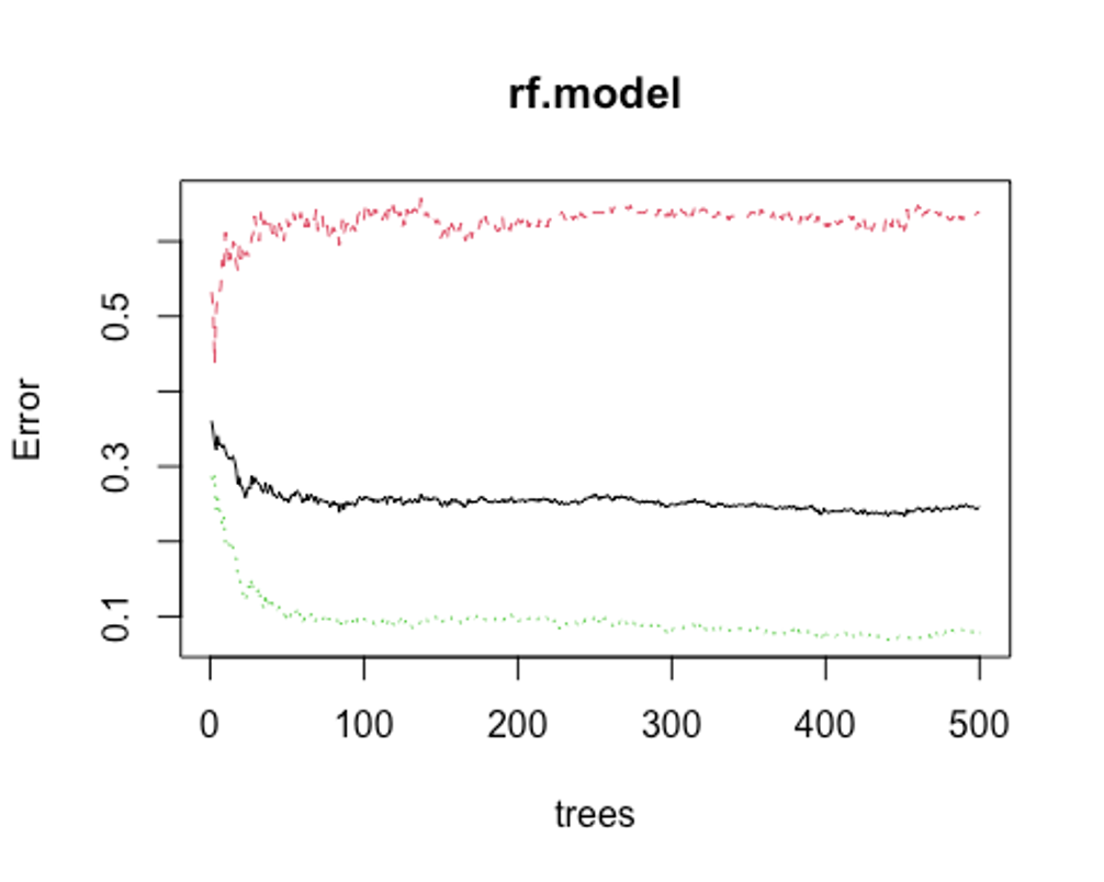
which.min(rf.model$err.rate[, 1])
## [1] 440
모형 정확도를 최적화 하기에 필요한 트리수가 440개면 된다는 결과를 얻었다.
- 다시 모형을 만들어 보자.
set.seed(123)
rf.model2 <- randomForest(credit_risk ~., data = train, ntree = 440)
rf.model2
##
## Call:
##  randomForest(formula = credit_risk ~ ., data = train, ntree = 440)
##                Type of random forest: classification
##                      Number of trees: 440
## No. of variables tried at each split: 3
##
##         OOB estimate of  error rate: 23.43%
## Confusion matrix:
##      bad good class.error
## bad   80  130  0.61904762
## good  34  456  0.06938776
OOB오차율이 24.57%에서 23.43%로 약간 떨어졌다.
- test데이터로 어떤 결과가 나오는지 보자.
rf.fit <- predict(rf.model2, newdata = test, type = 'class')
rf.fit <- as.factor(rf.fit)
rf.confusion <- confusionMatrix(rf.fit, test$credit_risk, positive = 'good')
rf.confusion
## Confusion Matrix and Statistics
##
##           Reference
## Prediction bad good
##       bad   28   13
##       good  62  197
##
##                Accuracy : 0.75
##                  95% CI : (0.697, 0.798)
##     No Information Rate : 0.7
##     P-Value [Acc > NIR] : 0.03224
##
##                   Kappa : 0.2951
##
##  Mcnemar's Test P-Value : 2.981e-08
##
##             Sensitivity : 0.9381
##             Specificity : 0.3111
##          Pos Pred Value : 0.7606
##          Neg Pred Value : 0.6829
##              Prevalence : 0.7000
##          Detection Rate : 0.6567
##    Detection Prevalence : 0.8633
##       Balanced Accuracy : 0.6246
##
##        'Positive' Class : good
##
rf.confusion$byClass
##          Sensitivity          Specificity       Pos Pred Value
##            0.9380952            0.3111111            0.7606178
##       Neg Pred Value            Precision               Recall
##            0.6829268            0.7606178            0.9380952
##                   F1           Prevalence       Detection Rate
##            0.8400853            0.7000000            0.6566667
## Detection Prevalence    Balanced Accuracy
##            0.8633333            0.6246032
Accuracy : 0.750, Kappa : 0.295, F1-score : 0.840의 성능이 나왔다.
- 성능을 좀 더 높여보자.
rf_mtry <- seq(4, ncol(train)*0.8, by = 2)
rf_nodesize <- seq(3, 8, by = 1)
rf_sample_size <- nrow(train) * c(0.7, 0.8)
rf_hyper_grid <- expand.grid(mtry = rf_mtry,
                             nodesize = rf_nodesize,
samplesize = rf_sample_size)- 설정된 파라미터를 바탕으로 모형을 적합한다.
rf_oob_err <- c()
for(i in 1:nrow(rf_hyper_grid)) {

  model <- randomForest(credit_risk ~., data = train,
                        mtry = rf_hyper_grid$mtry[i],
                        nodesize = rf_hyper_grid$nodesize[i],
                        samplesize = rf_hyper_grid$samplesize[i])

  rf_oob_err[i] <- model$err.rate[nrow(model$err.rate), 'OOB']
}- 최적의 하이퍼 파라미터를 보자.
rf_hyper_grid[which.min(rf_oob_err), ]
##    mtry nodesize samplesize
## 17 6 6 490- 위의 파라미터를 토대로 모형을 만들자.
rf_best_model <- randomForest(credit_risk ~., data = train,
                              mtry = 6,
                              nodesize = 6,
                              samplesize = 490,
                              proximity = TRUE,
importance = TRUE)- 변수 중요도를 보자.
varImpPlot(rf_best_model, type = 1)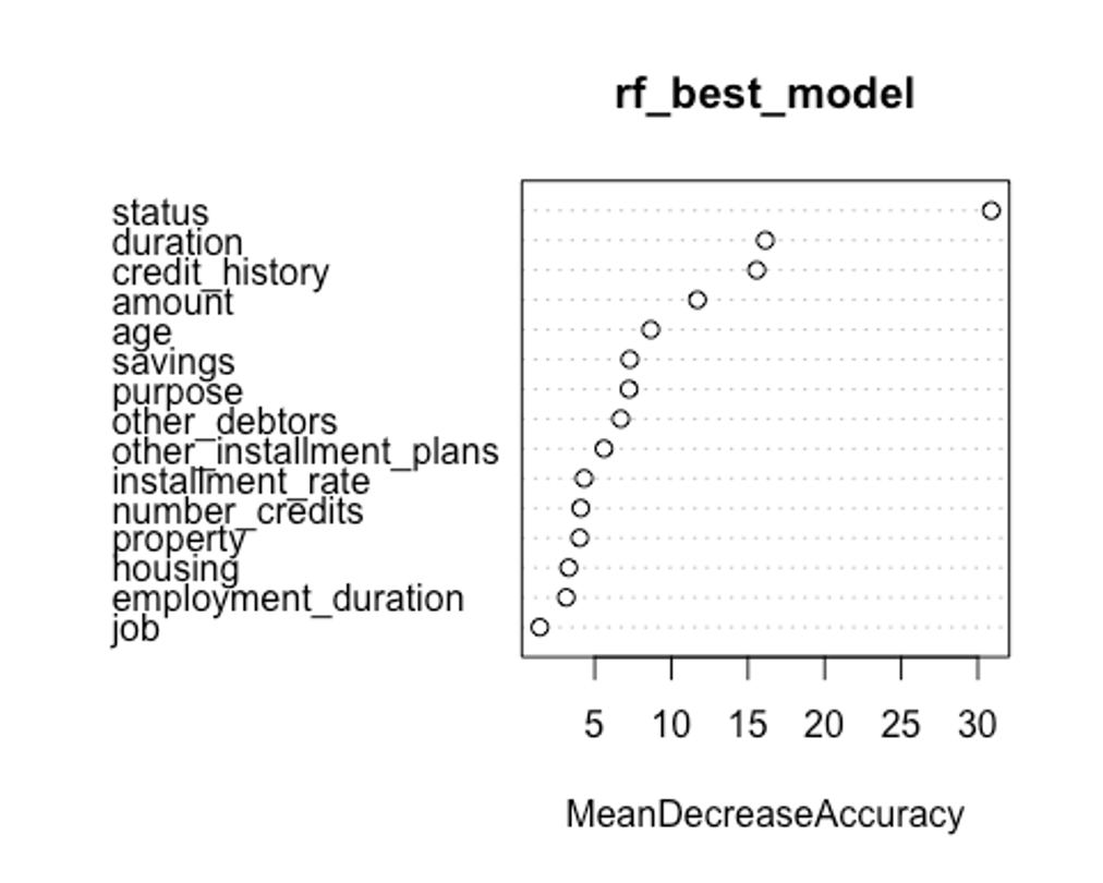
- type을 바꿔서 변수 중요도를 보자.
varImpPlot(rf_best_model, type = 2)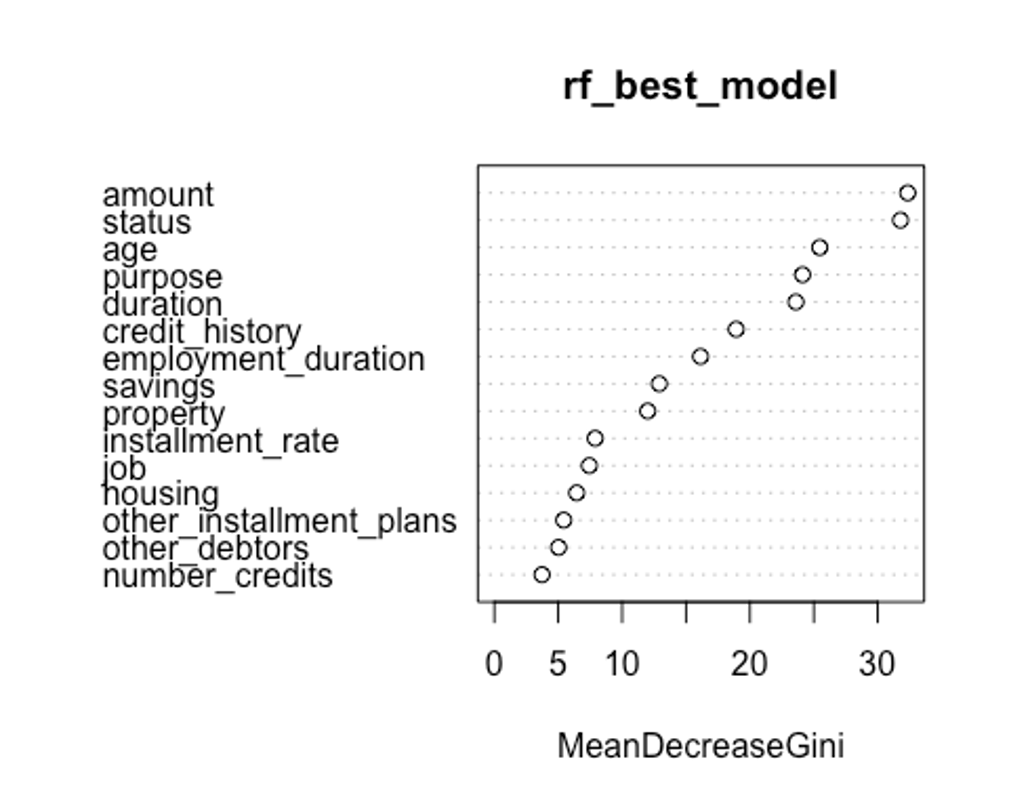
첫번째 plot을 보자. 변수의 값을 랜덤하게 섞었다면, 모델의 정확도가 감소하는 정도를 측정한다.(type = 1)
변수를 랜덤하게 섞는다는 것은 해당 변수가 예측에 미치는 모든 영향력을 제거하는 것을 의미한다. 정확도는 OOB데이터로부터 얻는다. 이는 결국 교차 타당성과 같은 효과를 얻는다.
두번째 plot을 보자. 특정 변수를 기준으로 분할이 일어난 모든 노드에서 불순도 점수의 평균 감소량을 측정한다.(type = 2)
이 지표는 해당 변수가 노드의 불순도를 개선하는데 얼마나 기여했는지를 나타낸다.
그러나 이 지표는 학습데이터를 기반으로 측정되기 때문에 OOB데이터를 가지고 계산한 것에 비해 믿을만하지 못하다.
우리의 plot에서 첫번째와 두번째 plot의 변수 중요도 순서가 다소 다른 것을 볼 수 있는데, OOB데이터로부터 정확도 감소량을 측정한 첫번째 plot이 더 믿을만하다.
- predict()함수로 예측을 해보자.
rf.predict <- predict(rf_best_model, newdata = test, type = 'class')
rf.predict <- as.factor(rf.predict)
rf.best.confusion <- confusionMatrix(rf.predict, test$credit_risk, positive = 'good')
rf.best.confusion
## Confusion Matrix and Statistics
##
##           Reference
## Prediction bad good
##       bad   32   19
##       good  58  191
##
##                Accuracy : 0.7433
##                  95% CI : (0.69, 0.7918)
##     No Information Rate : 0.7
##     P-Value [Acc > NIR] : 0.05608
##
##                   Kappa : 0.3025
##
##  Mcnemar's Test P-Value : 1.488e-05
##
##             Sensitivity : 0.9095
##             Specificity : 0.3556
##          Pos Pred Value : 0.7671
##          Neg Pred Value : 0.6275
##              Prevalence : 0.7000
##          Detection Rate : 0.6367
##    Detection Prevalence : 0.8300
##       Balanced Accuracy : 0.6325
##
##        'Positive' Class : good
##
rf.best.confusion$byClass
##          Sensitivity          Specificity       Pos Pred Value
##            0.9095238            0.3555556            0.7670683
##       Neg Pred Value            Precision               Recall
##            0.6274510            0.7670683            0.9095238
##                   F1           Prevalence       Detection Rate
##            0.8322440            0.7000000            0.6366667
## Detection Prevalence    Balanced Accuracy
##            0.8300000            0.6325397
Accuracy : 0.743, Kappa : 0.303, F1-score : 0.832의 성능이 나왔다. F1-score를 성능 평가의 기준으로 본다면 기본 랜덤 포레스트 모델보다 성능이 떨어졌다.
- scaled_train, scaled_test데이터를 사용하고, 하이퍼 파라미터를 조정해 성능을 좀 더 높여보자.
rf_mtry <- seq(1, 12, by = 2)
rf_nodesize <- seq(2, 8, by = 1)
rf_sample_size <- seq(350, 700, by = 25)
rf_hyper_grid <- expand.grid(mtry = rf_mtry,
                             nodesize = rf_nodesize,
samplesize = rf_sample_size)- 설정된 파라미터를 바탕으로 모형을 적합한다.
rf_oob_err <- c()
for(i in 1:nrow(rf_hyper_grid)) {

  model2 <- randomForest(credit_risk ~., data = scaled_train,
                        mtry = rf_hyper_grid$mtry[i],
                        nodesize = rf_hyper_grid$nodesize[i],
                        samplesize = rf_hyper_grid$samplesize[i])

  rf_oob_err[i] <- model2$err.rate[nrow(model2$err.rate), 'OOB']
}- 최적의 하이퍼 파라미터를 보자.
rf_hyper_grid[which.min(rf_oob_err), ]
##     mtry nodesize samplesize
## 176 3 3 450- 위의 파라미터를 토대로 모형을 만들자.
rf_best_model2 <- randomForest(credit_risk ~., data = scaled_train,
                              mtry = 3,
                              nodesize = 6,
                              samplesize = 525,
                              proximity = TRUE,
importance = TRUE)- predict()함수로 예측을 해보자.
rf.predict2 <- predict(rf_best_model2, newdata = scaled_test, type = 'class')
rf.predict2 <- as.factor(rf.predict2)
rf.best.confusion2 <- confusionMatrix(rf.predict2, scaled_test$credit_risk, positive = 'good')
rf.best.confusion2
## Confusion Matrix and Statistics
##
##           Reference
## Prediction bad good
##       bad   29   17
##       good  61  193
##
##                Accuracy : 0.74
##                  95% CI : (0.6865, 0.7887)
##     No Information Rate : 0.7
##     P-Value [Acc > NIR] : 0.07228
##
##                   Kappa : 0.2804
##
##  Mcnemar's Test P-Value : 1.123e-06
##
##             Sensitivity : 0.9190
##             Specificity : 0.3222
##          Pos Pred Value : 0.7598
##          Neg Pred Value : 0.6304
##              Prevalence : 0.7000
##          Detection Rate : 0.6433
##    Detection Prevalence : 0.8467
##       Balanced Accuracy : 0.6206
##
##        'Positive' Class : good
##
rf.best.confusion2$byClass
##          Sensitivity          Specificity       Pos Pred Value
##            0.9190476            0.3222222            0.7598425
##       Neg Pred Value            Precision               Recall
##            0.6304348            0.7598425            0.9190476
##                   F1           Prevalence       Detection Rate
##            0.8318966            0.7000000            0.6433333
## Detection Prevalence    Balanced Accuracy
##            0.8466667            0.6206349
Accuracy : 0.740, Kappa : 0.280, F1-score : 0.832의 성능이 나왔다. 성능이 더 좋아지지 않았다.
- 기본 랜덤포레스트 모형의 ROC그래프를 그려보자.
plot(perf.earth, col = 1)
plot(perf.knn, col = 2, add = TRUE)
plot(perf.svm, col = 3, add = TRUE)

rf.pred <- predict(rf.model2, newdata = test, type = 'prob')
head(rf.pred)
##           bad      good
## 2  0.09772727 0.9022727
## 4  0.22045455 0.7795455
## 10 0.31818182 0.6818182
## 15 0.26363636 0.7363636
## 22 0.32272727 0.6772727
## 23 0.57045455 0.4295455
rf.pred.good <- rf.pred[, 2]
pred.rf <- prediction(rf.pred.good, test$credit_risk)
perf.rf <- performance(pred.rf, 'tpr', 'fpr')

plot(perf.rf, col = 4, add = TRUE)
legend(0.6, 0.6, c('MARS', 'KNN', 'SVM', 'RF'), 1:4)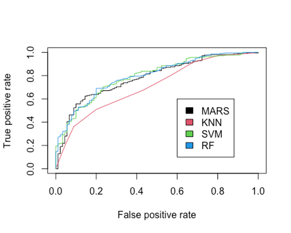
- AUC를 보자.
performance(pred.earth, 'auc')@y.values
## [[1]]
## [1] 0.7833333
performance(pred.knn, 'auc')@y.values
## [[1]]
## [1] 0.7093122
performance(pred.svm, 'auc')@y.values
## [[1]]
## [1] 0.7931217
performance(pred.rf, 'auc')@y.values
## [[1]]
## [1] 0.7965608
AUC를 성능 평가 지표의 기준으로 삼는다면 train, test데이터를 사용하고 하이퍼파라미터를 설정하지 않은 랜덤포레스트 모형이 가장 좋은 성능을 보인다.
XGBoost
- XGBoost모형을 만들어보자.
- scaled_train_dummy, scaled_test_dummy데이터를 사용한다.
- 그리드를 만들어 보자.
grid <- expand.grid(nrounds = seq(50, 200, by = 25),
                    colsample_bytree = 1,
                    min_child_weight = 1,
                    eta = c(0.01, 0.1, 0.3),
                    gamma = c(0.5, 0.25, 0.1),
                    subsample = 0.5,
max_depth = c(1, 2, 3))- trainControl인자를 조정한다. 여기서는 5-fold교차검증을 사용해보자.
cntrl <- trainControl(method = 'cv',
                      number = 5,
                      verboseIter = TRUE,
                      returnData = FALSE,
returnResamp = 'final')- train()함수를 이용해 데이터를 학습시킨다.
set.seed(123)
train.xgb <- train(x = scaled_train_dummy[, 1:56],
                   y = scaled_train_dummy[, 57],
                   trControl = cntrl,
                   tuneGrid = grid,
                   method = 'xgbTree')
## + Fold1: eta=0.01, max_depth=1, gamma=0.10, colsample_bytree=1, min_child_weight=1, subsample=0.5, nrounds=200 =1, min_child_weight=1, subsample=0.5, nrounds=200
...(생략)
## - Fold5: eta=0.30, max_depth=3, gamma=0.50, colsample_bytree=1, min_child_weight=1, subsample=0.5, nrounds=200
## Aggregating results
## Selecting tuning parameters
## Fitting nrounds = 125, max_depth = 2, eta = 0.1, gamma = 0.1, colsample_bytree = 1, min_child_weight = 1, subsample = 0.5 on full training set- 모형을 생성하기 위한 최적 인자들의 조합이 출력되었다.
- xgb.train()에서 사용할 인자 목록을 생성하고, 데이터 프레임과 입력피처의 행렬과 숫자 레이블을 붙힌 결과 목록으로 변환한다. 그런 다음, 피처와 식별값을 xgb.DMatrix에서 사용할 입력값으로 변환한다.
param <- list(objective = 'binary:logistic',
              booster = 'gbtree',
              eval_metric = 'error',
              eta = 0.1,
              max_depth = 2,
              subsample = 0.5,
              colsample_bytree = 1,
              gamma = 0.1)
x <- as.matrix(scaled_train_dummy[, 1:56])
y <- ifelse(scaled_train_dummy$credit_risk == 'good', 1, 0)
train.mat <- xgb.DMatrix(data = x, label = y)- 이제 모형을 만들어 보자.
set.seed(123)
xgb.fit <- xgb.train(params = param, data = train.mat, nrounds = 125)- 테스트 세트에 관한 결과를 보기 전에 변수 중요도를 그려 검토해보자.
- 항목은 gain, cover, frequency이렇게 세가지를 검사할 수 있다.
- gain은 피처가 트리에 미치는 정확도의 향상 정도를 나타내는 값, cover는 이 피처와 연관된 전체 관찰값의 상대 수치, frequency는 모든 트리에 관해 피처가 나타난 횟수를 백분율로 나타낸 값이다.
impMatrix <- xgb.importance(feature_names = dimnames(x)[[2]], model = xgb.fit)
impMatrix
##                                                        Feature        Gain
##  1:                                                     amount 0.157398006
##  2:                                                        age 0.111427759
##  3:                                                   duration 0.104828102
##  4:          status.... >= 200 DM / salary for at least 1 year 0.098779805
##  5:                                 status.no checking account 0.045890670
##  6:     credit_history.all credits at this bank paid back duly 0.043147072
##  7:                                             purpose.others 0.041527741
##  8:                       employment_duration.4 <= ... < 7 yrs 0.027726437
##  9:                                          purpose.car (new) 0.025369274
## 10:                                               housing.rent 0.024689123
## 11:                                         installment_rate.L 0.024615982
## 12:                             property.unknown / no property 0.024431661
## 13:    credit_history.critical account/other credits elsewhere 0.022071490
## 14:                         savings.unknown/no savings account 0.018883356
## 15:                                     savings.... >= 1000 DM 0.017799799
## 16:             credit_history.delay in paying off in the past 0.014739744
## 17:                                            purpose.repairs 0.012970326
## 18:                                    other_debtors.guarantor 0.012083905
## 19:    credit_history.existing credits paid back duly till now 0.011969521
## 20:                                           housing.for free 0.009955575
## 21:                                       property.real estate 0.009706637
## 22:                       employment_duration.1 <= ... < 4 yrs 0.009638779
## 23:                              job.skilled employee/official 0.009508778
## 24:                               other_installment_plans.none 0.009203559
## 25:                                         installment_rate.C 0.008579032
## 26:                                 employment_duration.< 1 yr 0.008388248
## 27:                                           number_credits.C 0.008293946
## 28:                                   job.unskilled - resident 0.006975516
## 29:                                          status.... < 0 DM 0.006723607
## 30:                                    status.0<= ... < 200 DM 0.006703870
## 31:                                 other_debtors.co-applicant 0.005636576
## 32: credit_history.no credits taken/all credits paid back duly 0.005447164
## 33:                               employment_duration.>= 7 yrs 0.005332335
## 34:                                         installment_rate.Q 0.005039385
## 35:                                                housing.own 0.005016942
## 36:                                purpose.furniture/equipment 0.004801123
## 37:                                      savings.... <  100 DM 0.004398813
## 38:                                         other_debtors.none 0.003846762
## 39:                                         purpose.car (used) 0.003631957
## 40:                               savings.100 <= ... <  500 DM 0.003357928
## 41:             job.manager/self-empl./highly qualif. employee 0.003339993
## 42:                                      property.car or other 0.003102056
## 43:                             other_installment_plans.stores 0.002855790
## 44:                                         purpose.retraining 0.002484107
## 45:                               other_installment_plans.bank 0.002402886
## 46:                             employment_duration.unemployed 0.002156045
## 47:                                           number_credits.L 0.001982209
## 48:         property.building soc. savings agr./life insurance 0.001140608
##                                                        Feature        Gain
##            Cover   Frequency
##  1: 0.1736933229 0.184065934
##  2: 0.1056685043 0.123626374
##  3: 0.1090901321 0.096153846
##  4: 0.0577161464 0.041208791
##  5: 0.0305699703 0.021978022
##  6: 0.0393700708 0.032967033
##  7: 0.0300374259 0.032967033
##  8: 0.0287408217 0.027472527
##  9: 0.0375002598 0.030219780
## 10: 0.0194150689 0.024725275
## 11: 0.0172320423 0.027472527
## 12: 0.0225202902 0.021978022
## 13: 0.0270201868 0.021978022
## 14: 0.0212742631 0.021978022
## 15: 0.0217733109 0.019230769
## 16: 0.0202348286 0.016483516
## 17: 0.0129862878 0.010989011
## 18: 0.0169555023 0.013736264
## 19: 0.0116250093 0.013736264
## 20: 0.0135117563 0.010989011
## 21: 0.0082403339 0.008241758
## 22: 0.0047013343 0.010989011
## 23: 0.0092542970 0.010989011
## 24: 0.0118169056 0.008241758
## 25: 0.0120544813 0.016483516
## 26: 0.0088895999 0.008241758
## 27: 0.0088333155 0.013736264
## 28: 0.0085558879 0.010989011
## 29: 0.0084992173 0.010989011
## 30: 0.0072959114 0.005494505
## 31: 0.0105030702 0.008241758
## 32: 0.0080729294 0.008241758
## 33: 0.0066758786 0.005494505
## 34: 0.0070290268 0.008241758
## 35: 0.0047924115 0.008241758
## 36: 0.0071471322 0.005494505
## 37: 0.0061498666 0.005494505
## 38: 0.0064975358 0.005494505
## 39: 0.0070939874 0.005494505
## 40: 0.0067544992 0.005494505
## 41: 0.0073590498 0.005494505
## 42: 0.0019204633 0.005494505
## 43: 0.0028404522 0.002747253
## 44: 0.0036840250 0.005494505
## 45: 0.0035308398 0.002747253
## 46: 0.0029040537 0.002747253
## 47: 0.0013373337 0.008241758
## 48: 0.0006309599 0.002747253
##            Cover   Frequency
xgb.plot.importance(impMatrix, main = 'Gain by Feature')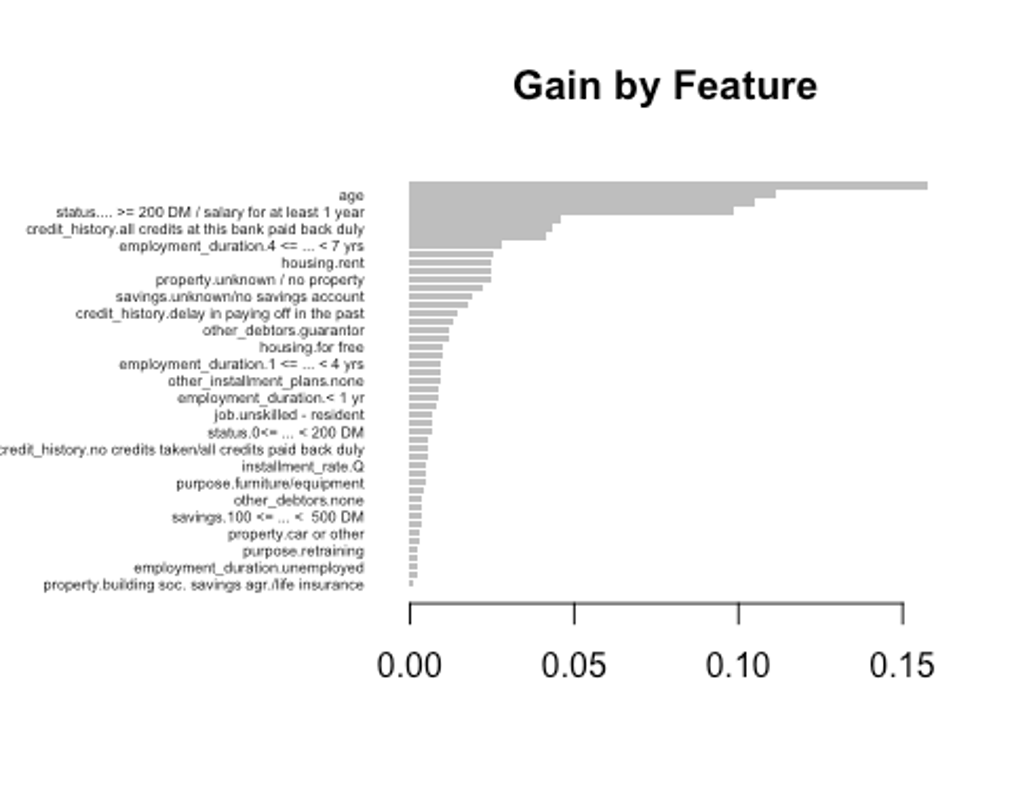
- 다음으로 scaled_test_dummy데이터에 관한 수행 결과를 보자.
library(InformationValue)
##
## Attaching package: 'InformationValue'
## The following object is masked from 'package:genridge':
##
##     precision
## The following objects are masked from 'package:caret':
##
##     confusionMatrix, precision, sensitivity, specificity
pred <- predict(xgb.fit, x)
optimalCutoff(y, pred)
## [1] 0.5027472
testMat <- as.matrix(scaled_test_dummy[, 1:56])
y.test <- ifelse(scaled_test_dummy$credit_risk == 'good', 1, 0)
xgb.test <- predict(xgb.fit, testMat)
confusionMatrix(y.test, xgb.test, threshold = 0.5027472)
##    0   1
## 0 41  22
## 1 49 188
1 - misClassError(y.test, xgb.test, threshold = 0.5027472)
## [1] 0.7633
약 76.91%의 정확도를 보였다.
- F1-score를 계산해보자.
Precision <- 188 / (22 + 188)
Recall <- 188 / (49 + 188)
f1 <- (2*Precision*Recall) / (Precision + Recall)
f1
## [1] 0.8411633
F1-score는 0.841이다.
- ROC커브를 그려보자.
plotROC(y.test, xgb.test)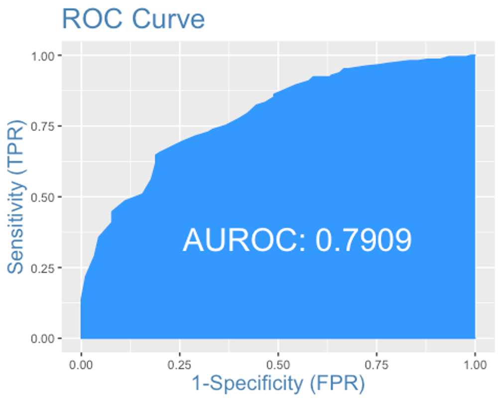
AUC는 0.791로 SVM모형과 랜덤포레스트 모형과 거의 비슷하다.
앙상블
- 앙상블 분석을 해보자.
- 데이터는 scaled_train, scaled_test데이터를 사용하자.
- 먼저 필요한 패키지들을 불러오자
library(caretEnsemble)
##
## Attaching package: 'caretEnsemble'
## The following object is masked from 'package:ggplot2':
##
##     autoplot
library(caTools)
library(mlr)
## Loading required package: ParamHelpers
## Warning message: 'mlr' is in 'maintenance-only' mode since July 2019.
## Future development will only happen in 'mlr3'
## (<https://mlr3.mlr-org.com>). Due to the focus on 'mlr3' there might be
## uncaught bugs meanwhile in {mlr} - please consider switching.
##
## Attaching package: 'mlr'
## The following object is masked _by_ '.GlobalEnv':
##
##     f1
## The following object is masked from 'package:e1071':
##
##     impute
## The following object is masked from 'package:ROCR':
##
##     performance
## The following object is masked from 'package:caret':
##
##     train
library(HDclassif)
library(gbm)
## Loaded gbm 2.1.8
library(mboost)
## Loading required package: parallel
## Loading required package: stabs
##
## Attaching package: 'stabs'
## The following object is masked from 'package:mlr':
##
##     subsample
##
## Attaching package: 'mboost'
## The following object is masked from 'package:partykit':
##
##     varimp
## The following object is masked from 'package:ggplot2':
##
##     %+%
## The following objects are masked from 'package:psych':
##
##     %+%, AUC
## The following object is masked from 'package:pastecs':
##
## extract- 5-fold교차검증을 사용하자.
control <- trainControl(method = 'cv', number = 5,
                        savePredictions = 'final',
                        classProbs = TRUE,
summaryFunction = twoClassSummary)- 이제 모형을 학습시키자. rpart, MARS, knn을 사용해보자.
set.seed(123)
Models <- caretList(credit_risk ~., data = scaled_train,
                    trControl = control,
                    metric = 'ROC',
                    methodList = c('rpart', 'earth', 'knn'))
Models
## $rpart
## CART
##
## 700 samples
##  15 predictor
##   2 classes: 'bad', 'good'
##
## No pre-processing
## Resampling: Cross-Validated (5 fold)
## Summary of sample sizes: 560, 560, 560, 560, 560
## Resampling results across tuning parameters:
##
##   cp          ROC        Sens        Spec
##   0.02222222  0.7201895  0.32857143  0.9020408
##   0.02857143  0.5852527  0.11428571  0.9571429
##   0.03928571  0.5738338  0.07142857  0.9734694
##
## ROC was used to select the optimal model using the largest value.
## The final value used for the model was cp = 0.02222222.
##
## $earth
## Multivariate Adaptive Regression Spline
##
## 700 samples
##  15 predictor
##   2 classes: 'bad', 'good'
##
## No pre-processing
## Resampling: Cross-Validated (5 fold)
## Summary of sample sizes: 560, 560, 560, 560, 560
## Resampling results across tuning parameters:
##
##   nprune  ROC        Sens       Spec
##    2      0.6676871  0.0000000  1.0000000
##   18      0.7451895  0.3809524  0.8693878
##   35      0.7498542  0.3904762  0.8714286
##
## Tuning parameter 'degree' was held constant at a value of 1
## ROC was used to select the optimal model using the largest value.
## The final values used for the model were nprune = 35 and degree = 1.
##
## $knn
## k-Nearest Neighbors
##
## 700 samples
##  15 predictor
##   2 classes: 'bad', 'good'
##
## No pre-processing
## Resampling: Cross-Validated (5 fold)
## Summary of sample sizes: 560, 560, 560, 560, 560
## Resampling results across tuning parameters:
##
##   k  ROC        Sens       Spec
##   5  0.6803450  0.3761905  0.8591837
##   7  0.6905005  0.3238095  0.8551020
##   9  0.6962342  0.3047619  0.8857143
##
## ROC was used to select the optimal model using the largest value.
## The final value used for the model was k = 9.
##
## attr(,"class")
## [1] "caretList"- 데이터 프레임 안의 테스트 세트에서 ’good’에 관한 예측값을 얻어오자.
model_preds <- lapply(Models, predict, newdata = scaled_test, type = 'prob')
model_preds <- lapply(model_preds, function(x) x[, 'good'])
model_preds <- data.frame(model_preds)- stack으로 로지스틱 회귀 모형을 쌓아보자.
stack <- caretStack(Models, method = 'glm', metric = 'ROC',
                    trControl = trainControl(
                      method = 'boot', number = 5,
                      savePredictions = 'final',
                      classProbs = TRUE,
                      summaryFunction = twoClassSummary
                    ))
summary(stack)
##
## Call:
## NULL
##
## Deviance Residuals:
##     Min       1Q   Median       3Q      Max
## -2.2296  -0.8923   0.5065   0.7556   1.9016
##
## Coefficients:
##             Estimate Std. Error z value Pr(>|z|)
## (Intercept)   2.6837     0.2185  12.282  < 2e-16 ***
## rpart        -1.7680     0.4872  -3.629 0.000284 ***
## earth        -2.1098     0.4928  -4.282 1.85e-05 ***
## knn          -1.6765     0.5391  -3.110 0.001873 **
## ---
## Signif. codes:  0 '***' 0.001 '**' 0.01 '*' 0.05 '.' 0.1 ' ' 1
##
## (Dispersion parameter for binomial family taken to be 1)
##
##     Null deviance: 855.21  on 699  degrees of freedom
## Residual deviance: 722.61  on 696  degrees of freedom
## AIC: 730.61
##
## Number of Fisher Scoring iterations: 4
모형의 계수가 모두 유의하다.
- 앙상블에 사용된 학습자의 각 예측결과를 비교해보자.
prob <- 1 - predict(stack, newdata = scaled_test, type = 'prob')
model_preds$ensemble <- prob
colAUC(model_preds, scaled_test$credit_risk)
##                  rpart     earth       knn  ensemble
## bad vs. good 0.7144709 0.7701058 0.6968519 0.7653968
각 모형의 AUC를 봤을 때 앙상블 모형이 오히려 단독 MARS모형보다 성능이 떨어진다.
- 앙상블 모형으로 confusion matrix를 만들어보자.
class <- predict(stack, newdata = scaled_test, type = 'raw')
head(class)
## [1] good good good good good bad
## Levels: bad good
detach("package:InformationValue", unload = TRUE)
ensemble.confusion <- confusionMatrix(class, scaled_test$credit_risk, positive = 'good')
ensemble.confusion
## Confusion Matrix and Statistics
##
##           Reference
## Prediction bad good
##       bad   32   23
##       good  58  187
##
##                Accuracy : 0.73
##                  95% CI : (0.676, 0.7794)
##     No Information Rate : 0.7
##     P-Value [Acc > NIR] : 0.1417892
##
##                   Kappa : 0.2768
##
##  Mcnemar's Test P-Value : 0.0001582
##
##             Sensitivity : 0.8905
##             Specificity : 0.3556
##          Pos Pred Value : 0.7633
##          Neg Pred Value : 0.5818
##              Prevalence : 0.7000
##          Detection Rate : 0.6233
##    Detection Prevalence : 0.8167
##       Balanced Accuracy : 0.6230
##
##        'Positive' Class : good
##
ensemble.confusion$byClass
##          Sensitivity          Specificity       Pos Pred Value
##            0.8904762            0.3555556            0.7632653
##       Neg Pred Value            Precision               Recall
##            0.5818182            0.7632653            0.8904762
##                   F1           Prevalence       Detection Rate
##            0.8219780            0.7000000            0.6233333
## Detection Prevalence    Balanced Accuracy
##            0.8166667            0.6230159
앙상블 모형의 성능은 AUC : 0.765, Accuracy : 0.730, Kappa : 0.277, F1-score : 0.822이다.
Conclusion
- 모든 분석이 끝났다.
- 총 6개의 모형을 만들었고, 각 모형의 평가 지표가 어떻게 나왔는지 비교해보자.
| - | MARS | KNN | SVM | RandomForest | XGBoost | Ensemble |
|---|---|---|---|---|---|---|
| Accuracy | 0.740 | 0.740 | 0.767 | 0.750 | 0.769 | 0.730 |
| F1-score | 0.824 | 0.835 | 0.848 | 0.840 | 0.841 | 0.822 |
| Kappa | 0.330 | 0.253 | 0.354 | 0.295 | - | 0.277 |
| AUC | 0.783 | 0.709 | 0.793 | 0.797 | 0.791 | 0.765 |
6개 모형 중 어떤 모형을 선택해야 할까?
우선 Accuracy는 전체 데이터에서 올바르게 분류한 데이터의 비율인데 단순히 이 지표만 보고 모형을 선택해서는 안된다. 정확도의 역설이라고 불리는 bias에 관한 단점을 가지기 때문이다.
이런 단점을 보완한 평가 지표가 recall과 precision인데 이 둘은 서로 반비례하는 경향이 있으므로 둘의 조화평균을 사용하는 F1-score를 보자.
F1-score를 기준으로 방사 기저 함수 커널을 사용한 SVM모형이 가장 좋은 성능을 보이고 있다.
SVM모형은 데이터가 크면 훈련 속도가 급격히 느려진다는 단점이 있지만 우리의 경우 데이터가 그렇게 크지 않으므로 훈련에 긴 시간이 걸리지 않았다.
또한 AUC를 성능 평가의 기준으로 삼아도 SVM이 랜덤포레스트 모형과 거의 비슷하게 좋은 성능을 보이고 있으므로 최종 모형으로 SVM를 선택하겠다.
사용한 패키지
caret, pastecs, psych, PerformanceAnalytics, Fselector, GGally, gridExtra, gapminder, dplyr, class, kknn, e1071, MASS, reshape2, ggplot2, kernlab, corrplot, rpart, partykit, genridge, randomForest, xgboost, Boruta, caretEnsemble, caTools, mlr, HDclassif, earth, Formula, plotmo, plotrix, ROCR, InformationValue, gbm, mboost