#경고 무시, 모듈 호출
import warnings
warnings.filterwarnings(action='ignore')
import numpy as np
from sklearn.model_selection import train_test_split
from sklearn.datasets import load_digits

#데이터 준비
digits = load_digits()
y = digits.target == 9
X_train, X_test, y_train, y_test = train_test_split(
    digits.data, y, random_state=0)

• 위에서 보면, load_digits는 데이터는 0부터 9까지의 손으로 쓴 숫자 이미지
• digits는 딕셔너리 형태고, 거기서 digits.target은 거기서 타겟(즉, 레이블)로 [0~9]로 된 1차원 넘파이 배열. y는 그 중에 ==9로 조건을 걸어서, 9만 True인 불리언 배열.

from sklearn.dummy import DummyClassifier

dummy_majority = DummyClassifier(strategy = 'most_frequent').fit(X_train, y_train)

pred_most_frequent = dummy_majority.predict(X_test)
print("예측된 레이블의 고유값:", np.unique(pred_most_frequent))
print("테스트 점수: {:.2f}".format(dummy_majority.score(X_test, y_test)))

• DummyClassifier(): 실제로 학습 안하고, 단순한 규칙이나 통계 기반으로 예측하는 분류기. => 더 복잡한 머신러닝 모델의 성능을 상대 평가하기 위한 기준선(baseline) 설정.
• 여기서는 strategy='most_frequent'로 가장 빈번한 레이블을 예측값으로 사용. => fit으로 훈련 데이터의 레이블(y_train)을 학습. => 여기서 most_frequent 전략으로 설정되어 있기 때문에, True, False 중에 더 많이 나오는 False로 모든 레이블을 예측.
• 그래서 np.unique로 predict의 결과를 보면 모두 False, 그리고 그렇게만 해도 score는 90% 나온다. 0~9 중 대해 모두 9가 아니라고 예측을 했으므로(데이터셋의 비율이 균등하다)

from sklearn.tree import DecisionTreeClassifier
tree = DecisionTreeClassifier(max_depth=2).fit(
    X_train, y_train)
pred_tree = tree.predict(X_test)
print('테스트 점수: {:.2f}'.format(tree.score(X_test, y_test)))


from sklearn.linear_model import LogisticRegression

dummy = DummyClassifier(strategy='stratified').fit(X_train, y_train)
pred_dummy = dummy.predict(X_test)
print('dummy 점수: {:.2f}'.format(dummy.score(X_test, y_test)))

logreg = LogisticRegression(C=0.1, max_iter=1000).fit(X_train, y_train)
pred_logreg = logreg.predict(X_test)
print('logreg 점수: {:.2f}'.format(logreg.score(X_test, y_test)))

• 다음으로 Depth를 2로 한 DecisionTreeClassifier로 예측을 했을 때 92%의 예측이 나온다.
• 다음으로, DummyClassifier에서 stratified 전략으로. 이는 각 클래스의 레이블이 나타날 확률을 훈련 데이터셋에서의 그들의 상대적 빈도에 기반해 결정. 즉, True가 10%, False가 90%니까, 그냥 무작위로 True 10%, False 90%로 예측.
• LoggisticRegression으로 예측.
  여기서 C는 정규화 강도의 역수. C가 낮을수록 정규화 강도가 높아지고, C가 높을수록 정규화 강도가 낮아진다. => 정규화가 높으면 모델의 복잡도가 감소해서 과대적합 위험 줄어들지만, 과소 적합 위험 커진다.
  max_iter는 최대 반복 횟수로, 모델이 수렴할 때까지 최적화 알고리즘이 반복되는 최대 횟수 설정. 로지스틱 회귀는 강사 하강법을 수행하므로, 그 횟수. => 너무 낮으면 충분히 반복 못하지만, 너무 높으면 시간이 너무 길어진다.

2 오차 행렬(Confusion metrics)

from sklearn.metrics import confusion_matrix
confusion = confusion_matrix(y_test, pred_logreg)
print('오차 행렬:\n', confusion)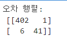

• 0행은 9가 아님 True, 9가 아님 False(9), 0열은 9가 아님 예측 True, 1열은 9가 아님 예측 False(9).

  따라서 [0, 0]은 True를 True로 예측, [0, 1]은 True를 False로 예측, [1, 0]은 False를 True로 예측, [1, 1]은 False를 False로 예측
  대각 행렬은 다 맞는 것.

print('빈도 기반 더미 모델:')
print(confusion_matrix(y_test, pred_most_frequent))
print('\n무작위 더미 모델:')
print(confusion_matrix(y_test, pred_dummy))
print('\n결정 트리:')
print(confusion_matrix(y_test, pred_tree))
print('\n로지스틱 회귀:')
print(confusion_matrix(y_test, pred_logreg))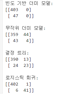

3 f1_score

• f1_score: 분류 문제에서 모델 성능 평가하는데 사용되는 지표 중 하나. 정밀도(Precision)과 재현율(Recall)의 조화 평균으로 계산, 클래스간 불균형이 있을 때 성능 평가에 유용하다.
  
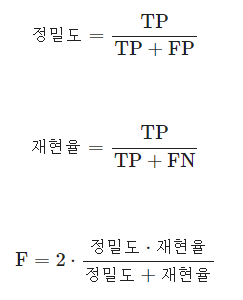
  (T가 실제 True, F가 실제 False)(P가 모델의 예측 True, N이 모델 예측 False)
• 정밀도(Precision): 모델이 True로 예측한 항목 중 실제 True인 비율.
• 재현율(Recall): 실제 True인 항목 중 모델이 True로 정확하게 예측한 비율.

from sklearn.metrics import f1_score

print('빈도 기반 더미 모델 f1 score: {:.2f}'.format(f1_score(y_test, pred_most_frequent)))
print('\n무작위 더미 모델 f1 score: {:.2f}'.format(f1_score(y_test, pred_dummy)))
print('\n결정 트리 f1 score: {:.2f}'.format(f1_score(y_test, pred_tree)))
print('\n로지스틱 회귀 f1 score: {:.2f}'.format(f1_score(y_test, pred_logreg)))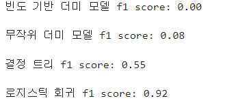

from sklearn.metrics import classification_report

print(classification_report(y_test, pred_most_frequent, 
                            target_names=['9 아님', '9'], zero_division=0))

print(classification_report(y_test, pred_logreg, 
                            target_names=['9 아님', '9']))

• classification_report: 실제 데이터셋 배열, 모델의 예측 배열로 => 분류 모델의 성능 평가하는 메서드. 정밀도, 재현율, F1스코어, 각 클래스에 대한 지지도(support, 각 클래스에 실제로 속하는 데이터포인트수)를 포함한 보고서 생성.
  - target_names는 대상 클래스의 이름 설정. 여기선 True를 9 아님, False를 9로.
  - zero_division=0은 0으로 나누는 경우 거기 0을 할당. 재현율, 정밀도, F1 스코어 등 계산할 때 분모 0이 될 때 그냥 0으로. 어떤 클래스에 대한 예측이 전혀 없을 때 발생.
  
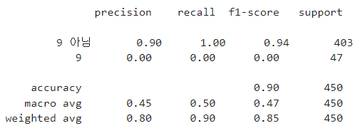
• support: 각 클래스에 실제로 속하는 데이터 포인트의 수. 9 아님에 403개, 9에 47개의 사례.
• accuracy: 전체 데이터 중 모델이 올바르게 예측한 데이터 포인트 비율.
• macro avg: 각 클래스에 대한 성능 지표의 단순 평균.
• weighted avg: 각 클래스으 ㅣsupport를 고려한 성능 지표의 가중 평균.

4 피마 인디언 당뇨병 데이터 분석

#모듈 호출
import pandas as pd
import matplotlib.pyplot as plt
from sklearn.model_selection import train_test_split
from sklearn.metrics import accuracy_score, precision_score, recall_score, roc_auc_score
from sklearn.metrics import f1_score, confusion_matrix, precision_recall_curve, roc_curve
from sklearn.preprocessing import StandardScaler
from sklearn.linear_model import LogisticRegression

#데이터 호출
diabetes_data = pd.read_csv('../data/diabetes.csv')

#데이터 파악 => 1이 당뇨병, 0이 당뇨병 아님
print(diabetes_data['Outcome'].value_counts())
diabetes_data.head()
diabetes_data.info() #null 값 없다

• 아래는 캐글에서 다른 사람이 해놓은 걸 참고한? 메서드들.

def get_clf_eval(y_test, pred=None, pred_proba=None):
    confusion = confusion_matrix( y_test, pred)
    accuracy = accuracy_score(y_test , pred)
    precision = precision_score(y_test , pred)
    recall = recall_score(y_test , pred)
    f1 = f1_score(y_test,pred)
    # ROC-AUC
    roc_auc = roc_auc_score(y_test, pred_proba)
    print('오차 행렬')
    print(confusion)
    # ROC-AUC print
    print('정확도: {0:.4f}, 정밀도: {1:.4f}, 재현율: {2:.4f},\
    F1: {3:.4f}, AUC:{4:.4f}'.format(accuracy, precision, recall, f1, roc_auc))

• 3개의 매개변수를 받는다. y_test는 실제값, pred는 모델이 예측한 분류값, pred_proba는 모델이 예측한 확률값.
• 오차행렬 confusion metrics, 정확도 accuracy, 정밀도 precision, 재현율 recall, f1스코어를 각각 계산.
• roc_auc_score: ROC-AUC(Receiver Operating Characteristic Curve) 아래의 면적으로 1에 가까울수록 좋은 성능이다. => 여기서 pred_proba가 필요. 나머지는 다 pred만.
• 구한 각각의 지표를 모두 print하는 메서드

# 데이터 준비
X = diabetes_data.iloc[:, :-1]
y = diabetes_data.iloc[:, -1]
X_train, X_test, y_train, y_test = train_test_split(
    X, y, test_size = 0.2, random_state = 156, stratify=y)
    
#로지스틱 회귀로 학습
lr_clf = LogisticRegression()
lr_clf.fit(X_train, y_train)
pred = lr_clf.predict(X_test)
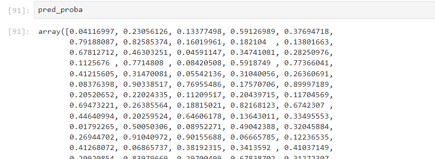
pred_proba = lr_clf.predict_proba(X_test)[:, 1]

get_clf_eval(y_test, pred, pred_proba)

• LogisticRegression은 여러 데이터를 바탕으로 y를 이진분류. 여기서는 당뇨병이 1인지 0인지.
• lr_clf.predict(): X_test에 대해서 각 값이 어떤지 1차원 배열로 예측을 반환.
• lr_clf.predict_proba(): 각 클래스의 예측 확률을 반환. 즉, 모델이 각 클래스에 속한다고 예측하는 확률을 각각 반환.
  
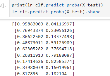
  => 여기서 [:, 1]이므로 2번째 클래스에 속한다고 여겨지는 확률을 1차원 배열로.
  
• 위에 만들어 놓은 메서드로 각 스코어를 반환한다.

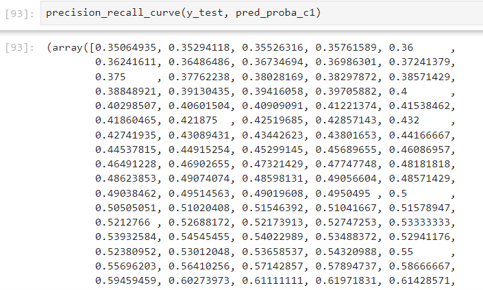
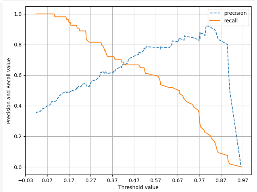
def precision_recall_curve_plot(y_test=None, pred_proba_c1=None):
    precisions, recalls, thresholds = precision_recall_curve( y_test, pred_proba_c1)
    # X축을 threshold값으로, Y축은 정밀도, 재현율 값으로 각각 Plot 수행
    #정밀도는 점선으로 표시
    plt.figure(figsize=(8,6))
    threshold_boundary = thresholds.shape[0]
    plt.plot(thresholds, precisions[0:threshold_boundary], linestyle='--', label='precision')
    plt.plot(thresholds, recalls[0:threshold_boundary],label='recall')
    # threshold 값 X 축의 Scale을 0.1 단위로 변경
    start, end = plt.xlim()
    plt.xticks(np.round(np.arange(start, end, 0.1),2))
    plt.xlabel('Threshold value'); plt.ylabel('Precision and Recall value')
    plt.legend(); plt.grid()
    plt.show()

• 매개변수: 실제 데이터값 배열 y_test,
  pred_proba_c1은 위에서 구한 pred_proba. 즉, predict_proba에서 2번째 클래스에 속할 확률의 배열.
• precision_recall_curve: y_test와 pred_proba_c1을 입력 받아서, 3개의 배열을 반환. 1 정밀도 값(precision), 재현율(recall), 정밀도와 재현율의 임계값. => 그것들을 각각의 변수에 넣는다.
  => 일반적으로 임계값을 높이면 정밀도는 증가하고, 재현율은 감소한다.
• 임계값(threshold)란? 분류기의 예측 확률을 클래스 레이블로 변환하는 경계값. 기본적으로 0.5를 임계값으로 사용하지만, 비지니스 요구나 문제 맥락에 따라 달라진다. 예를 들면, 질병 진단에선 질병이 있는 걸 없다고 예측하는 것의 비용이 훨씬 커진다.
  분류 모델이 각 샘플에 대해 클래스에 속할 확률을 제공하면, 각 임계값에서 정밀도와 재현율이 어떻게 되는지를 파악할 수 있다.
  => 여기서 임계값을 낮추면 더 많은 샘플을 양성 클래스로 분류해서, 정밀도 감소하고 재현율 올라간다(더 많은 샘플을 True로 분류하므로, 실제 True인 항목 중에서는 True로 예측한 갯수가 올라가지만, 모델이 True로 예측한 항목 중엔 False도 더 섞인다)
  (정밀도(Precision): 모델이 True로 예측한 항목 중 실제 True인 비율.
  재현율(Recall): 실제 True인 항목 중 모델이 True로 정확하게 예측한 비율. )
  
• 이제 그림을 그린다. threshold_boundary = thresholds.shape[0]로 하고 plt.plot(thresholds, precisions[0:threshold_boundary], linestyle='--', label='precision')로 하는 이유는, thresholds보다 precisions와 recalls가 항상 1개 더 많은 요소를 가지고 있기 때문. thresholds는 임계값들만 포함하지만, 정밀도와 재현율은 모든 걸 양성으로 분류하는(임계값이 0인 경우)의 스코어 포함. (임계값이 100인 경우, 모두 음성으로 분류하는 경우는 의미가 없어서 안들어간다)
• 어쨌든 thresholds값을 X축으로, Y축에 precisions와 recalls를 그리고, 각각 점선, 실선으로 그린다.
• plt.xlim()은 X축의 한계값을 2개 반환 => start, end 변수에 넣는다. => plt.xticks(): X축 눈금 설정. np.arange()로 start~end까지 0.1 간격으로 설정 후, np.round(, 2)로 소수점 둘째자리까지 반올림.

pred_proba_c1 = lr_clf.predict_proba(X_test)[:, 1]
precision_recall_curve_plot(y_test, pred_proba_c1)

• 위에 만든 메서드 활용
  

#그림 그려서 파악
plt.hist(diabetes_data['Glucose'], bins=100)

zero_features = ['Glucose', 'BloodPressure', 'SkinThickness', 'Insulin', 'BMI']

#전체 데이터 건수
total_count = diabetes_data['Glucose'].count()
#피처별로 반복하면서 데이터 값이 0인 데이터 건수 추출하고, 퍼센트 계산
for feature in zero_features:
    zero_count = diabetes_data[diabetes_data[feature] == 0][feature].count()
    print('{0} 0 건수는 {1}, 퍼센트는 {2:.2f} %'.format(feature, zero_count, 
        100*zero_count/total_count))

# zero_features 리스트 내부에 저장된 개별 피처들에 대해서 0값을 평균값으로 대체 
diabetes_data[zero_features] = \
diabetes_data[zero_features].replace(0, diabetes_data[zero_features].mean())

• 그림 그려서 분포 대충 파악
• 먼저 위의 for문은, 5개의 features에 대해, 0으로 들어간 값이 몇 개인지 꺼낸다.
• 그리고 각 값에 대해 그 열의 평균값으로 대체한다.

X = diabetes_data.iloc[:, :-1]
y = diabetes_data.iloc[:, -1]
scaler = StandardScaler()
X_scaled = scaler.fit_transform(X)

X_train, X_test, y_train, y_test = train_test_split(
    X_scaled, y, test_size = 0.2, random_state = 156, stratify=y)

• 이렇게 평균으로 0을 채운 값을 SS로 표준화. 여기서 y는 0, 1이 이진분류이므로 필요 없다.

lr_clf = LogisticRegression()
lr_clf.fit(X_train, y_train)
pred = lr_clf.predict(X_test)

pred_proba = lr_clf.predict_proba(X_test)[:, 1]
get_clf_eval(y_test, pred, pred_proba)

• 똑같이 로지스틱 회귀. => 결과가 평균 채우고 표준화 전보다 좋아졌다.

from sklearn.preprocessing import Binarizer

def get_eval_by_threshold(y_test , pred_proba_c1, thresholds):
    # thresholds 리스트 객체내의 값을 차례로 iteration하면서 Evaluation 수행.
    for custom_threshold in thresholds:
        binarizer = Binarizer(threshold=custom_threshold).fit(pred_proba_c1)
        custom_predict = binarizer.transform(pred_proba_c1)
        print('임곗값:',custom_threshold)
        get_clf_eval(y_test , custom_predict, pred_proba_c1)

• y 실제값과, pred_proba[:, 1] 값과, thresholds를 받는다.
• Binarizer(threshold=값): sklearn의 전처리 도구로, 지정된 임곗값을 기준으로 연속형 변수롤 0 또는 1로 변환한다. => 여기 위의 thresholds 를 돌려서 하나씩 넣는다.
• Binarizer는 단순히 임곗값을 기준으로 데이터 이진화하는 모델이라 별도의 학습 과정이 필요 없고, 여기서의 fit은 단순히 pred_proba_c1의 데이터 구조를 파악하는 용도.
• binarizer.transform()으로 값을 이진으로 실제로 바꾸고, 그걸 custom_predict로 집어넣는다.
• 그 각각의 모델에 대해 성능을 get_clf_eval로 출력한다.

5 자전거 문제

#데이터 준비
bike_df = pd.read_csv('../data/bike_train.csv')
print(bike_df.shape)
bike_df.head(3)
bike_df.info()

#datetime 열을 string에서 datetime으로 바꾸고, 각 연월일시를 추출해서 칼럼으로
bike_df['datetime'] = bike_df.datetime.apply(pd.to_datetime)
bike_df['year'] = bike_df.datetime.apply(lambda x: x.year)
bike_df['month'] = bike_df.datetime.apply(lambda x: x.month)
bike_df['day'] = bike_df.datetime.apply(lambda x: x.day)
bike_df['hour'] = bike_df.datetime.apply(lambda x: x.hour)
print(bike_df.info())
bike_df.head()

#필요 없는 열을 drop
drop_columns = ['datetime', 'casual', 'registered']
bike_df.drop(drop_columns, axis=1, inplace=True)
bike_df.head()

y_target = bike_df['count']
X_features = bike_df.drop(['count'], axis=1, inplace=False)

X_train, X_test, y_train, y_test = train_test_split(
    X_features, y_target, test_size = 0.3, random_state=0)
lr_reg = LinearRegression()
lr_reg.fit(X_train, y_train)
pred = lr_reg.predict(X_test)
evaluate_regr(y_test, pred)

• 파일을 정제
• y로 count를 넣고, X로 count 외의 값들을 넣는다.
• 그리고 데이터 나누고 => LinearRegression => fit => predict 똑같다.
• 마지막의 evaluate_regr은 RMSLE, RMSE, MSE를 출력하도록, 우리가 정의한 함수. 기존 있는 함수 X.

import numpy as np
from sklearn.metrics import mean_squared_error, r2_score, mean_absolute_error, mean_squared_log_error
origin = np.array([1, 2, 3, 2, 3, 5, 4, 6, 5, 6, 7])
pred = np.array([1, 1, 2, 2, 3, 4, 4, 5, 5, 7, 7])
MAE =  mean_absolute_error(origin, pred)
# MAE = 0.45454545454545453
MSE = mean_squared_error(origin, pred)
# MSE = 0.45454545454545453
RMSE = np.sqrt(MSE)
# RMSE = 0.674199862463242
MSLE = mean_squared_log_error(origin, pred)
# MSLE = 0.029272467607503516
RMSLE = np.sqrt(mean_squared_log_error(origin, pred))
# RMSLE = 0.1710919858073531
R2 = r2_score(origin, pred)
# R2 = 0.868421052631579

• mean_absolute_error: MAE, 평균 절대 오차. 예측값과 실제값 차이의 절대값의 평균.
• mean_squared_error: MSE, 평균 제곱 오차. 예측값과 실제값 차이의 제곱값의 평균. 큰 오차에 가중치가 더 크게 부여.
• np.squrt(MSE): RMSE(Root MSE), MSE의 제곱근. 마찬가지로 큰 오차에 더 큰 가중치 부여되지만, 오차 단위가 실제값과 동일해져서 해석이 더 쉽다.
• mean_squared_log_error: MSLE, 평균 제곱 로그 오차. 예측값과 실제값에 1을 더한 => 로그를 취한 값 => 의 차이 => 의 제곱 => 의 평균. 0에 가까운 값들에서 발생하는 큰 상대적 오차에 더 민감.
• np.sqrt(MSLE):RMSLE(Root MSLE). MSLE의 제곱근으로, 오차의 상대적 크기에 초점을 맞추고, 과대 예측과 과소 예측을 동일하게 취급.
• r2_score: R^2로 결정 계수. 1에 가까울수록 모델이 잘 설명하고 있는 것.
• np.log1p(): log(1+x)와 동일. log(0)은 정의되지 않지만, log1p(0)은 0으로 계산된다.

def get_top_error_data(y_test, pred, n_tops = 5):
    # DataFrame에 컬럼들로 실제 대여횟수(count)와 예측 값을 서로 비교 할 수 있도록 생성.
    result_df = pd.DataFrame(y_test.values, columns=['real_count'])
    result_df['predicted_count']= np.round(pred)
    result_df['diff'] = np.abs(result_df['real_count'] - result_df['predicted_count'])
    # 예측값과 실제값이 가장 큰 데이터 순으로 출력.
    print(result_df.sort_values('diff', ascending=False)[:n_tops])

• 실제값과 예측값 차이 한 눈에 보여주는 함수 만듦.

y_target.hist()

y_log_transform = np.log1p(y_target)
y_log_transform.hist()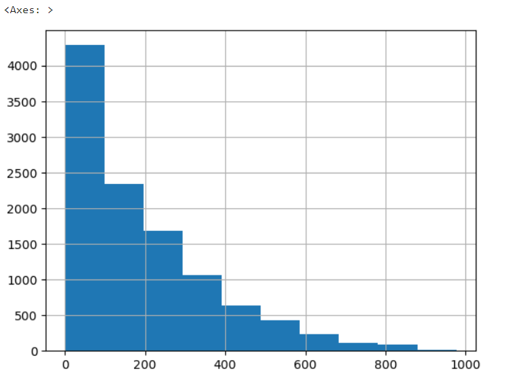

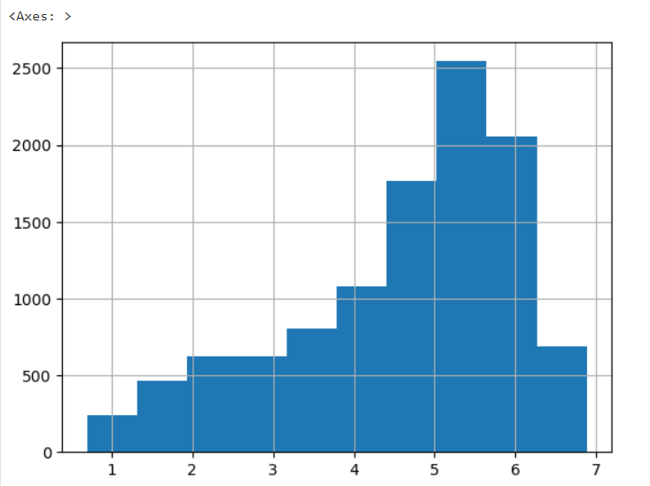
• 선형 회귀 같은 모델은 정규 분포에 가깝게 변환해야 더 잘 학습을 한다. => 한쪽으로 치우친 데이터는, log취하면 일반적으로 좀 잡힌다. => 이 상태로 적용하면 수치 좀 좋아지기도.

#타겟 컬럼인 count 값을 log1p로 log 변환
y_target_log = np.log1p(y_target)

#로그 변환된 y_target_log를 반영해 학습/테스트 데이터셋 분할
X_train, X_test, y_train, y_test = train_test_split(
    X_features, y_target_log, test_size=0.3, random_state=0)
lr_reg = LinearRegression()
lr_reg.fit(X_train, y_train)
pred = lr_reg.predict(X_test)
print(evaluate_regr(y_test, pred))

#테스트 데이터 셋의 Target 값은 log 변환되었으므로 expm1을 이용해 원래 스케일로
y_test_exp = np.expm1(y_test)
pred_exp = np.expm1(pred)
evaluate_regr(y_test_exp, pred_exp)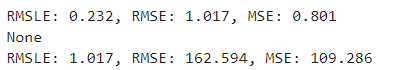

• y_target을 log로 스케일을 맞춘 후 => 다시 쪼개서 => LinearRegression() 모델을 만들어 fitting한다 => 그 로그 스케일을 다시 np.expm1으로 돌린다. => 그렇게 MSE 등을 구한다
• 스케일을 원래대로 돌리는 이유는 그래야 알기 편하기 때문에. 위에서 보듯이, 밑의 값들은 기존의 값보다 약간 개선된 값이지만, 위의 값들은 로그 스케일로 너무 작아져서 의미를 알아차리기 힘들다.

X_features_ohe = pd.get_dummies(X_features,
            columns=['year','month','hour', 'holiday',
                        'workingday','season','weather'])
X_train, X_test, y_train, y_test = train_test_split(
    X_features_ohe, y_target_log, test_size = 0.3, random_state=0)

• X에서 get_dummies를 이용해 칼럼의 값들을 각각 True, False로 바꾼다. => 원-핫 인코딩(One-hot encoding)을 적용. 원-핫 인코딩이란 범주형 변수를 각각 이진 벡터로 변환해서 기계 학습에 적용하는 것. 빨노파를 [1, 0, 0], [0, 1, 0], [0, 0, 1] 정도로.

def get_model_predict(model, X_train, X_test, y_train, y_test, is_expm1=False):
    model.fit(X_train, y_train)
    pred = model.predict(X_test)
    if is_expm1 :
        y_test = np.expm1(y_test)
        pred = np.expm1(pred)
    print('###',model.__class__.__name__,'###')
    evaluate_regr(y_test, pred)

lr_reg = LinearRegression()
ridge_reg = Ridge(alpha=10)
lasso_reg = Lasso(alpha=0.01)
for model in [lr_reg, ridge_reg, lasso_reg]:
    get_model_predict(model,X_train, X_test, y_train, y_test,is_expm1=True)

• 모델과, 데이터셋을 넣으면 성능 수치를 반환. is_expm1으로 기본 스케일로 돌려서 값을 반환하길 원하면 np.expm1으로 돌린다.
• 각 모델을 만들어서 for문으로 하나씩 돌려본다.

참고 자료

https://www.kaggle.com/c/bike-sharing-demand
https://www.kaggle.com/c/bike-sharing-demand/overview/evaluation
RMSLE(실제 값과 예측값의 오류를 로그로 변환한 뒤 RMSE를 적용) kaggle.comkaggle.com Bike Sharing Demand Forecast use of a city bikeshare s
https://daewonyoon.tistory.com/281
https://wikidocs.net/34063
https://hjryu09.tistory.com/33ystem
https://m.blog.naver.com/hajuny2903/222375600616