Packages

import numpy as np
import copy
import matplotlib.pyplot as plt
from testCases_v2 import *
from public_tests import *
import sklearn
import sklearn.datasets
import sklearn.linear_model
from planar_utils import plot_decision_boundary, sigmoid, load_planar_dataset, load_extra_datasets

%matplotlib inline

np.random.seed(2) # set a seed so that the results are consistent

%load_ext autoreload
%autoreload 2

Load Data

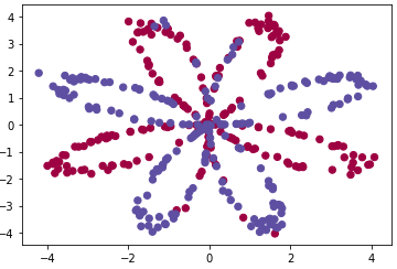
여기서는 2-클래스 데이터 세트인 "flower"를 사용할 것이다.

X,Y = load_plannar_dataset()

plt.scatter(X[0, :], X[1, :], c=Y, s=40, cmap=plt.cm.Spectral);

위 코드를 실행시켜 시각화하면 아래와 같이 출력된다.

X와 Y가 어떻게 생겼는지 확인해보자.

shape_X = X.shape     #shape of X
shape_Y = Y.shape     #shape of Y
m = X.shape[1]        #training examples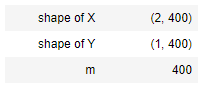 

400개의 샘플개수, 각각 2차원,1차원의 데이터셋이 400개씩 있다는 사실을 확인할 수 있다.

Logistic Regression

로지스틱 회귀를 사용해서 간단한 클래스 분류를 해 보자.

clf = sklearn.linear_model.LogisticRegressionCV();
clf.fit(X.T, Y.T);

plot_decision_boundary(lambda x: clf.predict(x), X, Y)
plt.title("Logistic Regression")

LR_predictions = clf.predict(X.T)
print ('Accuracy of logistic regression: %d ' % float((np.dot(Y,LR_predictions) + np.dot(1-Y,1-LR_predictions))/float(Y.size)*100) +
       '% ' + "(percentage of correctly labelled datapoints)")

위 출력 결과와 같이 47%라는 낮은 정확도가 나와서 이 데이터에는 선형회귀가 맞지 않는다. 뉴럴 네트워크로 트레이닝 해보자.

Neural Network model

1개의 hidden layer를 가진 Neural Network에서 다시 학습시켜보자.
우선 각각의 structure들을 정의하고 마지막에 모델을 구축하도록 하겠다.

layer_sizes

def layer_sizes(X, Y):
    n_x = X.shape[0]      #the size of input layer
    n_h = 4               #the size of hidden layer
    n_y = Y.shape[0]      #the size of output layer
    return (n_x, n_h, n_y)
    
(n_x, n_h, n_y) = layer_sizes(t_X, t_Y)

print("The size of the input layer is: n_x = " + str(n_x))
print("The size of the hidden layer is: n_h = " + str(n_h))
print("The size of the output layer is: n_y = " + str(n_y))

The size of the input layer is: n_x = 5
The size of the hidden layer is: n_h = 4
The size of the output layer is: n_y = 2
각 층에서 레이어의 개수를 알아보았다.

Initialize_parameters

이번에는 파라미터들을 초기화 해본다.

def initialize_parameters(n_x, n_h, n_y):
    np.random.seed(2)
    # we set up a seed so that your output matches ours although the initialization is random.
    
    W1 = np.random.randn(n_h, n_x)*0.01
    b1 = np.zeros((n_h, 1))
    W2 = np.random.randn(n_y, n_h)*0.01
    b2 = np.zeros((n_y, 1))
    
    parameters = {"W1": W1,
                  "b1": b1,
                  "W2": W2,
                  "b2": b2}
    return parameters
    
parameters = initialize_parameters(n_x, n_h, n_y)

print("W1 = " + str(parameters["W1"]))
print("b1 = " + str(parameters["b1"]))
print("W2 = " + str(parameters["W2"]))
print("b2 = " + str(parameters["b2"]))

Forward_propagation

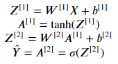
두 개의 레이어 층에서는 위 식을 따른다. 이를 이용해서 forward_propagation 함수를 완성한다.

def forward_propagation(X, parameters):
    W1 = parameters["W1"]
    b1 = parameters["b1"]
    W2 = parameters["W2"]
    b2 = parameters["b2"]
    
    Z1 = np.dot(W1,X) + b1
    A1 = np.tanh(Z1)
    Z2 = np.dot(W2,A1) + b2
    A2 = sigmoid(Z2)
    
    assert(A2.shape == (1, X.shape[1]))
    
    cache = {"Z1": Z1,
             "A1": A1,
             "Z2": Z2,
             "A2": A2}
    
    return A2, cache
    
A2, cache = forward_propagation(t_X, parameters)
print("A2 = " + str(A2))

A2의 벡터값을 얻을 수 있다.

Cost function

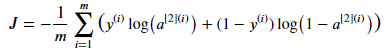
위 식을 이용하여 cost function을 계산해보자.

참고로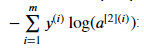
이 식은
logprobs = np.multiply(np.log(A2),Y)
cost = - np.sum(logprobs) 이렇게 나타낼 수 있다.

def compute_cost(A2, Y):
    m = Y.shape[1]      #number of example
    
    logprobs = np.multiply(np.log(A2),Y)+np.multiply((1-Y), np.log(1-A2))
    cost = -1/m*np.sum(logprobs)
    
    cost = float(np.squeeze(cost))  # makes sure cost is the dimension we expect. 
                                    # E.g., turns [[17]] into 17 
                                    
    return cost
    
cost = compute_cost(A2, t_Y)

Backward_propagation

다른 함수들보다 조금 복잡하긴 하지만, 천천히 따라가다보면 금방 구현해낼 수 있다. 공식은 아래를 참고한다.

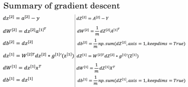
참고로, 𝑔[1]′(𝑍[1])는 (1 - np.power(A1, 2))를 사용해서 간단히 나타낼 수 있다. 구현해보자!

def backward_propagation(parameters, cache, X, Y):
    m = X.shape[1]
    
    W1 = parameters["W1"]
    W2 = parameters["W2"]
    
    A1 = cache["A1"]
    A2 = cache["A2"]
    
    dZ2 = A2 - Y
    dW2 = 1/m * np.dot(dZ2, A1.T)
    db2 = 1/m * np.sum(dZ2, axis=1, keepdims=True)
    dZ1 = np.dot(W2.T, dZ2) * (1 - np.power(A1, 2))
    dW1 = 1/m * np.dot(dZ1, X.T)
    db1 = 1/m * np.sum(dZ1, axis=1, keepdims=True)
    
    grads = {"dW1": dW1,
             "db1": db1,
             "dW2": dW2,
             "db2": db2}
    
    return grads

grads = backward_propagation(parameters, cache, t_X, t_Y)

Update parameters

위에서 구했던 loss function과 backward propagation을 이용하여 parameters들을 업데이트 하여 모델에 더 맞게 데이터들을 학습시키는 과정이다.

위 수식을 대입하여 업데이트 시켜주자.

def update_parameters(parameters, grads, learning_rate = 1.2):
    W1 = parameters["W1"]
    b1 = parameters["b1"]
    W2 = parameters["W2"]
    b2 = parameters["b2"]
    
    dW1 = grads["dW1"]
    db1 = grads["db1"]
    dW2 = grads["dW2"]
    db2 = grads["db2"]
    
    W1 = W1 - learning_rate*dW1
    b1 = b1 - learning_rate*db1
    W2 = W2 - learning_rate*dW2
    b2 = b2 - learning_rate*db2
    
    parameters = {"W1": W1,
                  "b1": b1,
                  "W2": W2,
                  "b2": b2}
    
    return parameters
parameters = update_parameters(parameters, grads)

parameters[]안에 각 값이 담기게 된다. 마지막으로 위의 함수들을 합쳐서 최종 모델을 만들어보자.

NN_Model

def nn_model(X, Y, n_h, num_iterations = 10000, print_cost=False):
    np.random.seed(3)
    n_x = layer_sizes(X, Y)[0]
    n_y = layer_sizes(X, Y)[2]
    
    parameters = initialize_parameters(n_x, n_h, n_y)
    
    for i in range(0, num_iterations):
        A2, cache = forward_propagation(X, parameters)
        cost = compute_cost(A2, Y)
        grads = backward_propagation(parameters, cache, X, Y)
        parameters = update_parameters(parameters, grads, learning_rate = 1.2)
        
        if print_cost and i % 1000 == 0:
            print ("Cost after iteration %i: %f" %(i, cost))
            
    return parameters
    
parameters = nn_model(t_X, t_Y, 4, num_iterations=10000, print_cost=True)

Predict

모델을 구현했으니, 예측을 하는 함수를 만들어야 한다. 0.5 이상 값이 나오면 True로, 아니면 False가 나오게 한다.

def predict(parameters, X):
    A2, cache = forward_propagation(X, parameters)
    predictions = A2 > 0.5
    
    return predictions
    
predictions = predict(parameters, t_X)

Test Model

테스트셋에 모델을 도입시켜 테스트해보자.

parameters = nn_model(X, Y, n_h = 4, num_iterations = 10000, print_cost=True)

plot_decision_boundary(lambda x: predict(parameters, x.T), X, Y)
plt.title("Decision Boundary for hidden layer size " + str(4))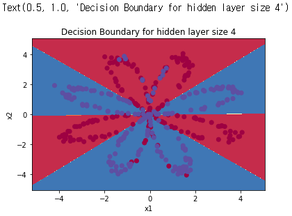

predictions = predict(parameters, X)
print ('Accuracy: %d' % float((np.dot(Y, predictions.T) + np.dot(1 - Y, 1 - predictions.T)) / float(Y.size) * 100) + '%')

출력되는 정확도는 90%로 로지스틱 회귀에서 얻었던 정확도보다 훨씬 높은 정확도를 갖고 있다.