🚀 Motivations

• The majority of extant Generation of 3D data works resort to regular represenations such as volumetric grids or collection of images

• However, these representations obscure the natural invariance of 3D shapes under geometric transformation ,and also suffer from a number of other issues.

🔑 Key Contribution

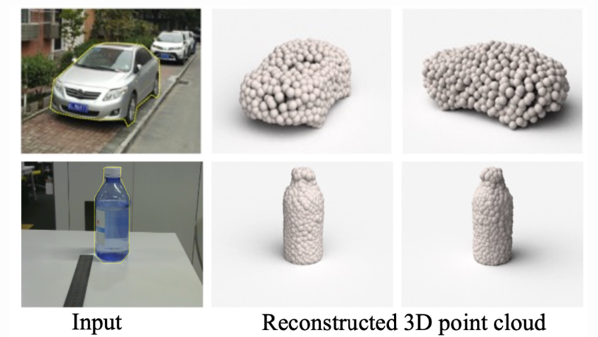
• This paper addresses the problem of generating the 3D geometry of an object based on a single image of that object.
  

• First to study the point set generation problem by deep learning
  (Generative networks for 3D geometry based on a point cloud representation.)

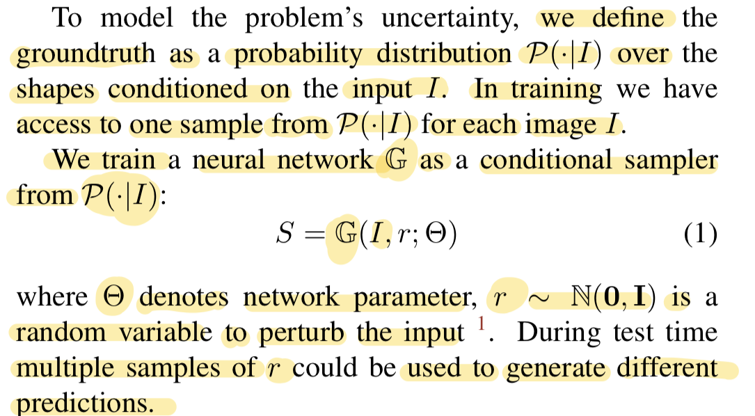
• Conditional shape sampler, capable of predicting multiple plausible 3D point clouds from an input image.

• Principled formulation and solution to address the groundtruth ambiguity issue for the 3D reconstruction from single image task.

📔 Notations

🔥 Challenges

• building a conditional generative network for point sets is challenging, due to unordered form of representation and the inherent ambiguity of groundtruth.

• This paper addresses 3 subproblems

1) Point set generator architecture
network with two prediction branches, one enjoys high flexibility in capturing complicated structures and the other exploits geomoetric continuity

2) Loss function for point set comparison
how to measure the distance between the prediction and groundtruth.
This paper introduces two distance metrics for point sets
-> the Chamfer distance(CD) & the Earth Mover's distance(EMD)
Both metrics are differentiable almost eveywhere and can be used as the loss function.

3) Modeling the uncertainty of groundtruth
Simply Using min function as a wrapper to the above proposed loss, or by a conditional variational autoencoder, Characterizing the ambiguity of groundtruth for a given input, and practically Generating multiple predictions are achieved.

⭐ Methods

1) Point Set Prediction Network

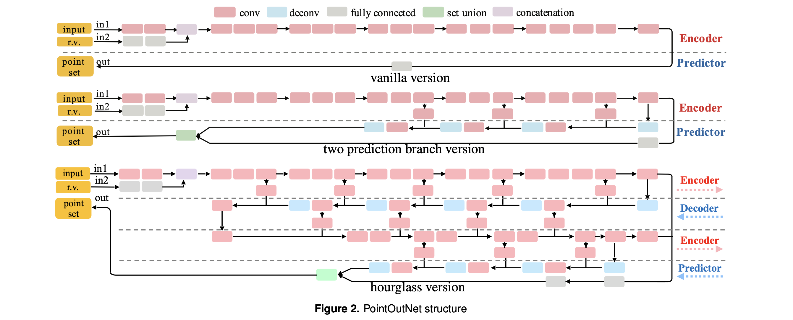
Network for point set prediction has an encoder stage and a predictor stage.

1-1) Vanila version

• Encoder
  -> Encoder maps the input pair of an image I and a random vector r into an embedding space.
  -> Composition of convolution and ReLU layers.
  -> Random vector r is subsumed so that it perturbs the prediction from the image I.

• Predictor
  -> Predictor outputs a shaps matrix M (N x 3), each row containing the coordinates of one point.
  -> Predictor generates the coordinats of N points through a fully connected network.

1-2) Two prediction branch version: Predictor branch is improved to better accomodate large and smooth sufaces.

Fully connected predictor as above can't make full use of natural geometric statics, since each point is predicted independently.

This version has two parallel predictor branches
fully-connected branch (fc) & deconvolution branch(deconv).

fc branch

• predicts N1 points as before.
• offer high flexibility, good performance at describing intricate stuructures.

deconv branch

• predicts a 3 channel image of size H x W, of which the three values at each pixel are the coordinates of a point, giving another H x W points.
• More friendly to large smooth sufaces, due to the spatial continuity induced by deconv and conv.

Their predictions are later merged together to form the whole set of points in M.
(Multiple skip links are added to boost information flow across encoder and predictor)

1-3) Hourglass version: Persuing better performance

• conducts encoding-decoding operations recurrently
• thus has stronger representation power and can mix global and local info better.

🤔 still needs to design a proper loss function for point set prediction, and enable the role r for multiple candidates prediction.

2) Distance Metric between Point Sets

• A crticical challenge is to design a good loss function for comparing the predicted point cloud and the groundtruth.
• For a distance d between subsets in ℝ^3, loss function takes the form
  
• This paper proposes two candidates: Chamfer distance (CD) and Earth Mover's Distance (EMD)

Chamfer distance

• Chamfer distance(CD) measures the squared distance between each point in one set to its nearest neighbor in the other set.
  
• For each point, the algorithm of CD finds the nearest neighbor in the other set and sums the squared distances up.
  -CD is differentiable and compared to EMD more efficient to compute.

Earth Mover's distance

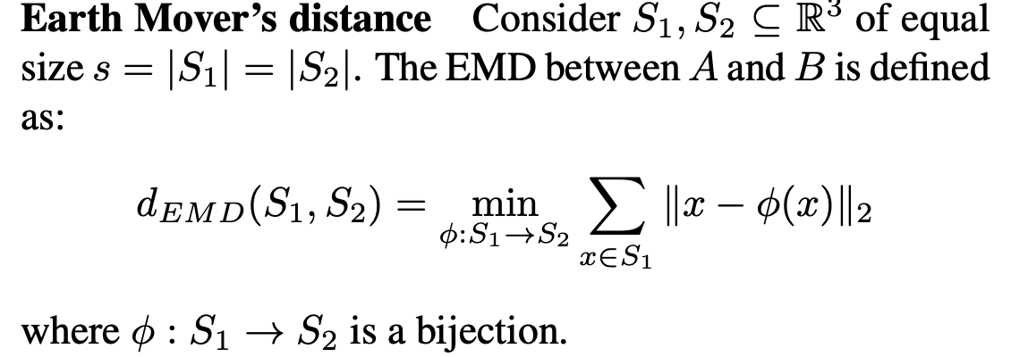
• The EMD distance solves an optimization problem.
• Thus EMD is differentiable almost everywhere.

Shape space

• Neural Networks inevitably encounter uncertainty in predicting the precise geometry of an object.
• Facing the inherent inability to resolve the shape recisely, neural networks tend to predict a "mean" shape averaging out the space of uncertainty.
• The mean shape carries the characteristics of the distance itself.
• EMD shows more meaningful average shape, but it is computaionally more expensive.
  

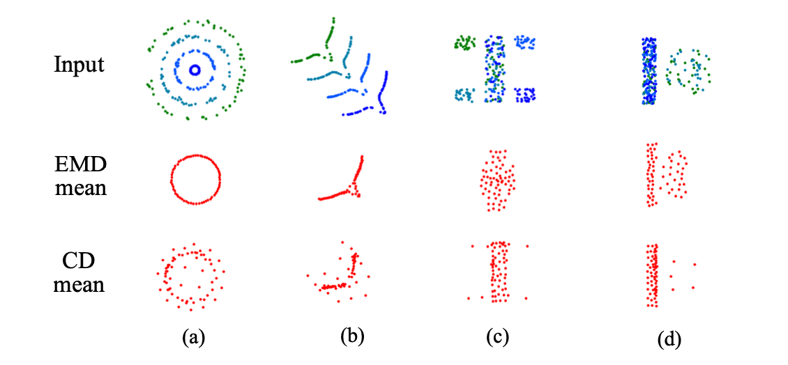
3) Generation of Multiple Plausible Shapes

• Ambiguity of the prediction arises at test time - the depth for visible parts is under-determined, and the geomotry for invisible parts has to be hallucinated by guessing.
• In as statistical view, reasonable predictions from the input image form a distribution.
• To better model the uncertainty or inherent ambiguity (e.g. unseen parts in the single view), we enable the system to generate distributional output.
• This paper expected random variable r passed to 𝔾 would help it explore the groundtruth distribution, in analogy to conditional GAN.
• This paper suggest the loss function 'MoN loss(Min-of-N loss)' for uncertainty modeling. Network is trained to minimize a MoN loss function.
  
  
• Any of the point set regression network versions can be plugged into the meta network below, incorporating the MoN logg.
  
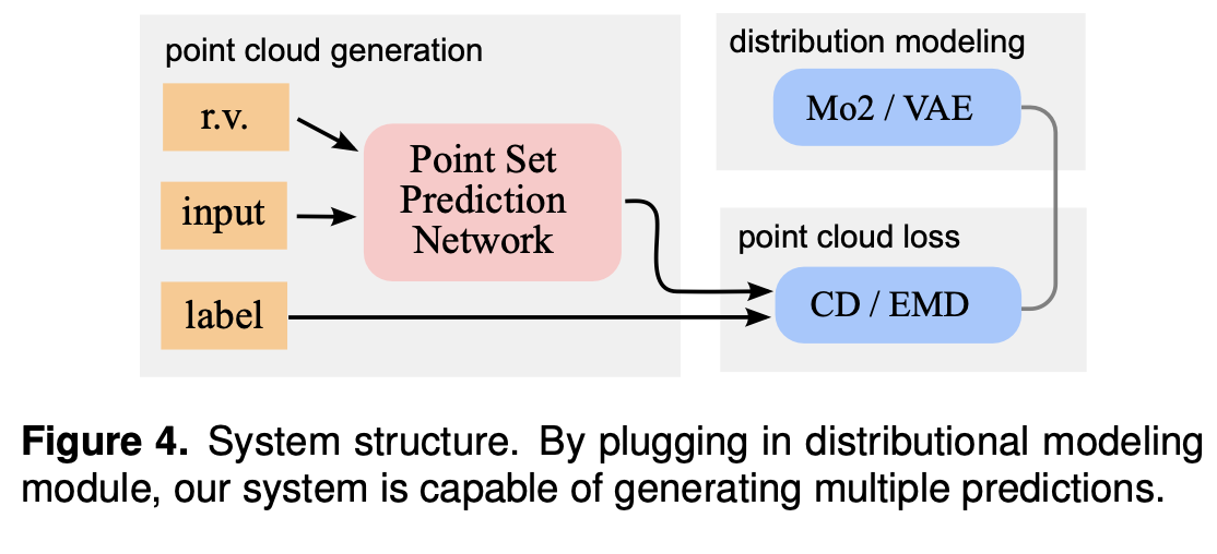
• An alternative way to achieve the conditional shape sampler is by a conditional variational autoencoder.
  
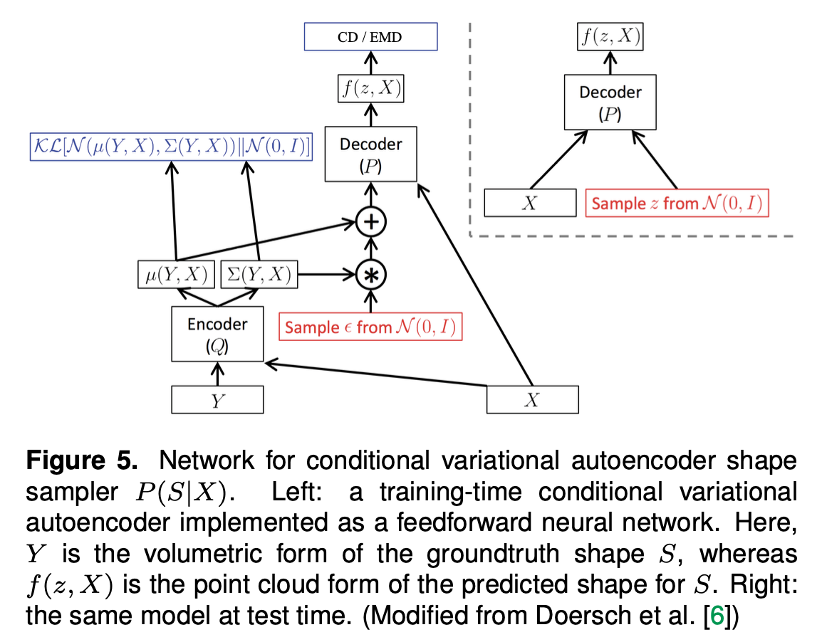
• Fig 5 shows the system architecture for training and testing a conditional variational autoencoder P(S|X) in paper's case.
• X: input image, S: point cloud representation of the groundtruth 3D shape.
• Each input image X will be augmented by a random variable that is conditioned on Y, which takes the volumetric representation of the groundtruth shape S.
• A 3D convolutional vetwork is used as the encoder Q.
• Therefore, a local proximity in the embedding space contains the variations of possible groundtruth 3D shapes.

👨🏻‍🔬 Experiment

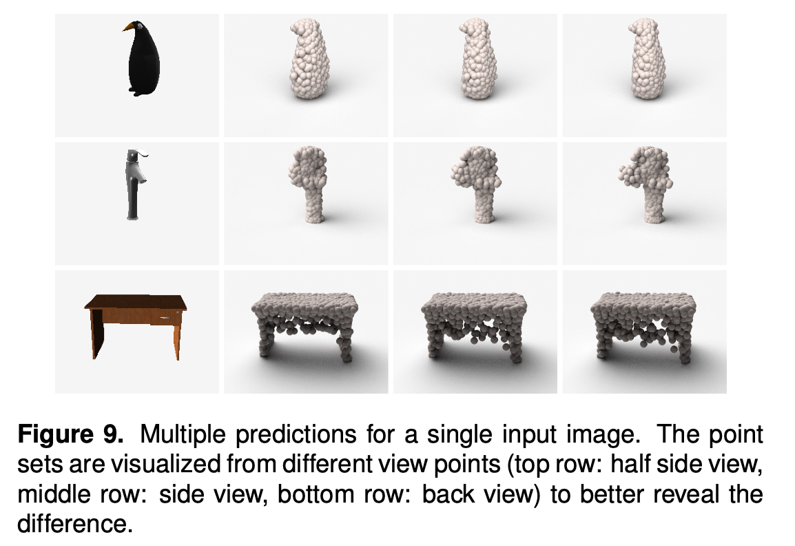
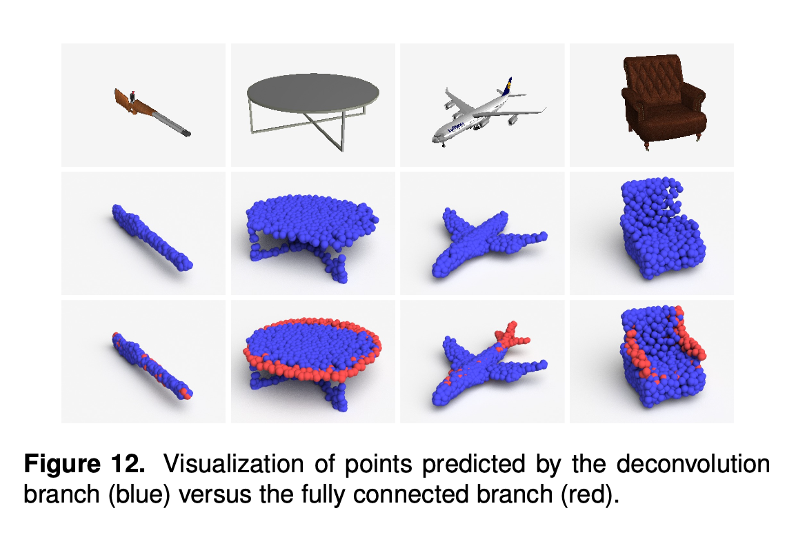
Effect of combining deconv and fc branches for reconstruction

• Deconv branch is in general good at capturing the "main body" of the object.
• Fully Connected branch complments the shape with more detailed components (e.g. tip of gun, tail of plane, arms of a sofa).
  -This reveals the complementary of the two branches.
  
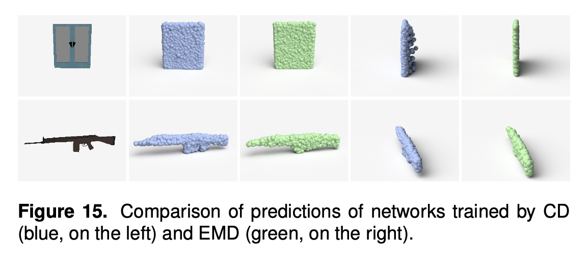
  Analysis of distance metrics
• Network trained by CD tends to scatter a few points in its uncertain area (e.g. behind the door), but is able to better preserve the detailed shape of the grip.
• Network trained by EMD produces more compact results, but sometimes overly shrinks local structures.