2024.03 arXiv, Gholami

• keyword: memory bandwidth, bottleneck

Introduction

• LLM의 main performance bottlenck은 (기존 computing에서) memory bandwidth이 되어가고 있다.
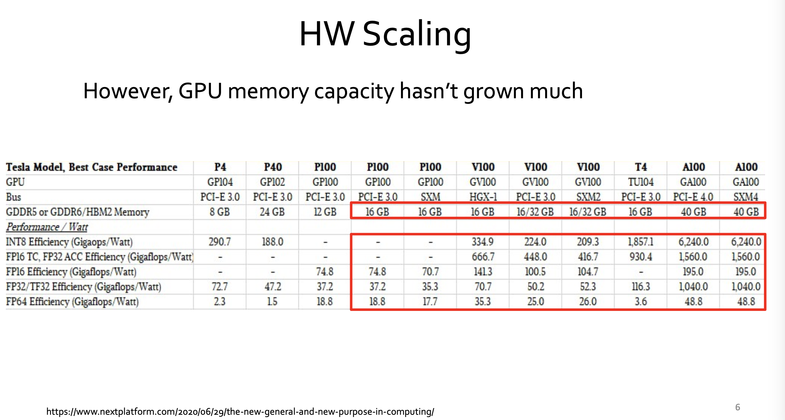
  (특히 LLM serving에서)

  • computing: 과거 20년 동안, 60,000X 이상 향상 peak server hardware FLOPS는 3.0x/2yrs로 scaling.
    $\\$
    $\\$
  • memory: 과거 20년 동안,
    DRAM은 100X 향상, 1.6x/2yrs로 scaling
    interconnect bandwidth는 30X 향상, 1.4x/2yrs로 scaling.

• LLM을 train하기 위해 필요한 연산량은 750x/2yrs로 증가하고 있다.

  • 이러한 exponention trend는 AI accelerator가 hardware의 peak compute를 증가하는데 focus하게 한다.
  • (often at the expense of simplifying other parts such as memory hierarchy. )

• operation(연산)을 완료하는데 걸리는 시간은 두 가지에 의존.

  • compute: arithmetic을 얼마나 빨리 수행할 수 있는지

  • memory bandwidth: hardware의 arithmetic units에 data를 얼마나 빨리 feed할 수 있는지.

• hardware가 computing(arithmetic)을 아무리 빠르게 하더라도, DRAM bandwidth 때문에 제한된다.

  • data는 Cache에 이미 있거나,
    DRAM에서 fetch해야 하거나

  • 80%의 데이터가 cache에 즉시 사용 가능한 상태로 있고
    단 20%만 DRAM에서 가져와야 한다고 해도,
    만약 이 20%의 cache-miss 데이터를 가져오는 데 5 cycles 이상 걸린다면,
    전체 operation 완료 시간은 전적으로 DRAM에 의해 제한된다.

• $\textcolor{red}{memory \ wall}$ 문제

  • capacity
  • bandwidth of memory transfer
  • latency (bandwidth보다 향상 어려움)

• different levels of "memory data transfer"

  • between 'compute logic' and 'on-chip memory'
  • between 'compute logic' and 'DRAM memory'
  • between 'different processors on different sockets'
  • 이 모든 case에 대해서, capacity와 data transfer speed는 hardware compute 성능보다 크게 뒤떨어져 있음.

• compute는 bottlececk이 아니다. memory가 bottleneck.

  • 최근 모델을 train 하는데 필요한 compte / FLOPs 는 750X/2yrs로 증가 (2018-2022) 했지만,
    compute는 bottleneck이 아니다. 특히 model serving에서.

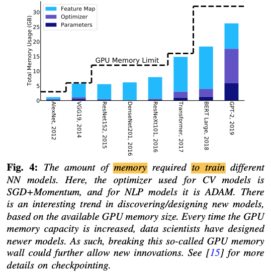
• single chip memory capacity << LLM size

  • LLM size는 410x/2yrs로 증가 (2018-2022)

  • 이는 single chip의 memory capacity를 초과.

  • 가능한 반문: single chip의 memory capacity와 bandwidth 문제를 해결하기 위해,
    distributed-memory parallelism을 사용해서 multiple accelerator들로 training/serving을 scaling out하면 되지 않냐?

    • 하지만, multiple process를 distributing하는 것도 memory wall 문제에 부딪힘.
      NN accelerator들 간에 data를 이동하는 communication bottleneck
      (on-chip data 이동보다 느리고 비효율적인)

  • model이 single chip에 fit하더라도,
    intra-chip memory transfer가 bottleneck.
    (from/to registers, L2 cache, global memory, etc.)

    • 최근의 specialized compute unit (Tensor core 같은) 발전으로, large set arithmetic 연산들은 몇 cycle 이내에 끝낸다.
    • 따라서 이러한 arithmetic unit들을 항상 활용(utilized) 상태로 유지하려면,
      대량의 data를 빠르게 공급(feed)해야 하는데, 바로 이 지점에서 chip memory bandwidth가 bottleneck.

Case Study

Transformer의 두 가지 architecture를 실험.
encoder architecture(e.g. BERT), decoder architecture(e.g. GPT)

A. Arithmetic Intensity

• Arithmetic Intensity의 필요성

  • performance bottleneck을 measure하기 위한 popular method는
    encoder-only, decoder-only model을 compute하기 위한 total number of FLOPs

  • 하지만, 이것만 놓고 보는 것은 잘못된 해석으로 이끌 수 있다.

  • operation의 arithmetic intensity를 봐야 한다.

• 

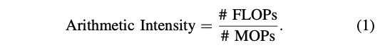
• Arithmetic Intensity: memory로부터 load되는 per byte(즉, data) 당 수행되는 num of FLOPs를 의미.
  (MOPs: Memory Operation)

B. Profiling

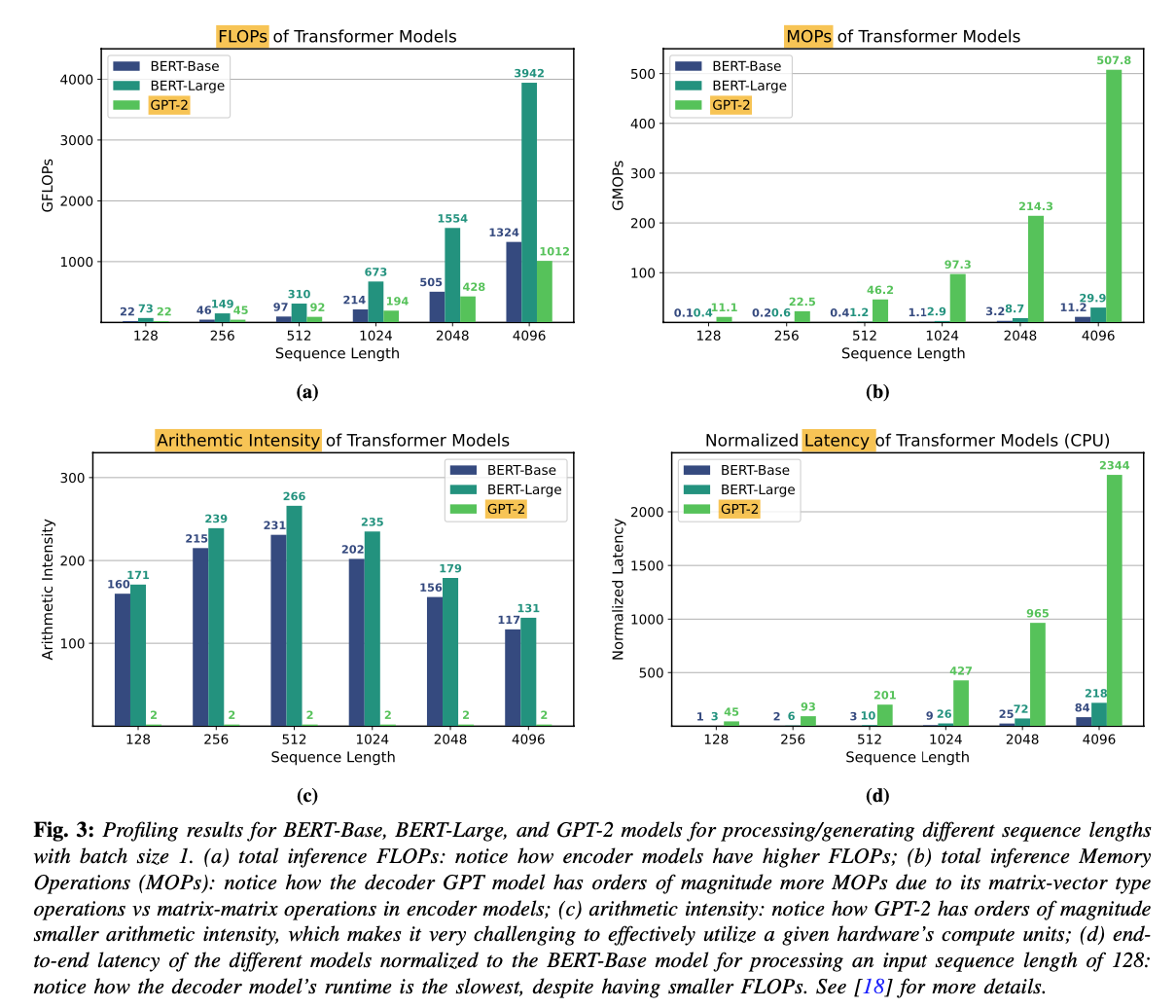
• Tansformer workloads의 bottleneck을 분석하기 위해,
  Transformer inference를 intel Gold 6242 CPU에서 profiling.

• 결과

  • 

  • decoder-only (GPT-2)의 latency가 encoder-only(BERT 계열)보다 훨씬 큼
    (각 sequence length에 대해서. BERT-Base와 GPT-2는 거의 동일한 model config를 갖고 있음에도)

  • 이는 GPT의 auto-regressive inference에 내재된
    higher memory operations와 lower arithmetic intensity of matrix-vector operations 때문.

    • deocder model

      • auto-regressive inference: 이전에 생성된 token들을 기반으로, 한 번에 하나의 token 생성.

      • 따라서, sequential하게, 각 step에서 matrix-vector multiplication 수행
        (weight matrix와 지금까지 생성된 token들의 hidden states(embeddings) 간의 multiplication)

      • 각 token마다 이전에 생성된 token들을 retrieve하기 위해 frequent한 memory access가 필요.

      • fewer computations relative to the amount of memory being accessed (= lower arithmetic intensity)

      • $\therefore$ bottleneck = memory bandwidth

    • encoder model

      • 모든 token들을 parallel로 처리.

      • 한 번에 matrix-matrix multiplication 수행.

      • larger data chunks and more computations per memory access (=high arithmetic intensity)

  • arithmetic intensity가 높은 model은 낮은 model보다 더 빠르게, (동일한, 혹은 더 많은 FLOPs에서도) 실행 가능하다.

  • 이는 decoder models (at low batch sizes)에서 major bottleneck은 compute가 아닌 memory wall임을 명확히 보여준다.

Promising Solutions for Breaking the Wall

A. Efficient Training Algorithms

challenge(for training NN models)와 promising approache들

• challenge 1: need for brute-force hyperparameter tuning.

  • learning rate, its annealing schedule, the number of iterations needed to converge...
  • 주요 원인: first-order SGD methods는 hyperparam tuning에 robust하지 않음.
  • promising approach: to use second- order stochastic optimization methods
  • AdaHessian
    • robust to hyperparameter tuning
    • 한계: 3–4× higher memory footprint
  • Zero framework from Microsoft
    • train 8× bigger models with the same memory capacity
      by removing/sharding redundant optimization state variables

• promising approach: reducing memory footprint &
  increasing the data locality of optimizatino algorithms,
  at the expense of performing computation

  • communication avoiding algorithms
    Minimizing communication in numerical linear algebra
  • rematerialization
    • only store/checkpoint a subset of activations during the forward pass,
      instead of saving all activations.
    • it reduces the feature map’s memory footprint.
    • rest of the activations could then be recomputed when needed
    • 
    • allow practitioners to train large models on single-chip memory rather than utilize distributed training, which is often difficult to set up

• promising approach: low-precision training에 robust한 optimization 알고리즘.

  • breakthrough in AI accelerators: half-precision (FP16) arithmetic 사용,
    instead of single precision
    • hardware compute capability 10× 이상 증가.
  • challenge: half-precision to INT8,
    without accuracy degradation
  • promising trend: mixture of FP8 and FP16 (and even most recently FP4)

B.Efficient Deployment

Model compression

• Approach 1: Quantization(reducing precision)

  • 현재 여기까지 가능
    • training에선 FP16 이하가 어렵지만,
      inference에선 ultra-low로 가능.
    • 현재 INT4까지는 accuracy 최소 영향으로 가능.
  • challenge: sub-INT4 precision은 매우 어렵고, 현재 활발한 연구 분야.

• Approach 2: Pruning(removing redundant parameters)

  • 현재 여기 까지 가능.

    • Structured sparsity: Up to 30% of neurons
    • Unstructured sparsity: Up to 80%

  • challenge: 이 이상으로 하는거.

• Approach 3: Design small LLMs

  • new frontiers
  • It’s not just size that matters: Small language models are also few-shot learners
  • Transformer 모델이 2017에 소개된 이후, LLM의 모델은 바뀌지 않음.
  • data랑 model size를 키우면서 LLM 모델의 능력이 점프했지만,
  • 최근엔 small LLM이 promising result를 보임.
  • model이 on-chip에 완벽하게 fit한다면, speedup과 energy 절약이 매우 어마어마함.

C.Rethinking the Design of AI Accelertators

• peak compute를 희생해서, compute/bandwidth trade-off를 달성할 수도 있음.

• CPU 구조는 최적화된 cache hierarchy 이미 사용.

  • 이것이 CPU가 GPU보다 bandwidth-bound 문제에 더 좋은 성능을 보이는 이유.

  • CPU의 challenge: peak compute capability (즉, FLOPS)가 GPU나 TPU와 같은 AI accelerator들보다 매우 낮음.

• AI accelerator들이 주로 maximum peak compute를 달성하도록 설계되었기 때문.

  • 더 많은 compute logic을 추가하기 위해 cache hierarchy와 같은 component들을 제거

• 가능한 대안

  • 더 효율적인 caching을 갖추기.
  • 더 높은 capacity의 DRAM (다양한 bandwidth를 가진 DRAM들의 hierarchy) 갖추기.
    • distributed-memory communication bottleneck들을 완화하는 데 도움.