• Sensitivity-based non-uniform Q

• Dense-and-Sparse decomposition (= outlier extraction)

  • sparse part: stores outliers and sensitivity weight values in an sparse format.

  • dense part: compact range to aid Q.

Motivation

• main bottleneck for LLM inference: memory bandwidth
  (rather than compute, specifically for single batch inference.)

  • LLaMA-65B: 130GB+ RAM for FP16 deployment >> current GPU capacity.

  • speed for load and store parameters

non-uniform Q

• uniform Q의 두 가지 main issue

  • LLM의 weight distribution은 non-uniform patterns

  • uniform Q의 main 이점은 efficient integer computation인 반면, memory bound한 end-to-end latency를 향상시키진 않음.

    • (Appendix A) recent hardware trends indicate that faster computation does not necessarily translate to improved end-to-end latency or throughput (Gholami et al., 2024), particularly in memory-bound tasks like generative LLM inference.

Dense-and-Sparse Decomposition

• Matrix를 dense, sparse로 decomposition하는 것은attention map decomposition에서 연구됨.

  • ScatterBrain, Vitality
  • leverage the fact that attention patterns often present low-rank characteristics with a few outliers

• dense-and-sparse decomposition 전략을 Q 성능을 높이기 위해서, weight matrics에 적용한 것이 우리가 처음

Memory Wall

• 아래 논문 기반으로 정리해 놓은 듯.

  • AI and Memory Wall(Gholami, 2024)
  • Full stack Optimization of Transformer Inference: a Survey(Kim, 2023)

• Inference behavior는 크게 두 가지 범주로 나눌 수 있음.

  • 계산 처리량에 의해 제한되는 compute-bound inference
  • 메모리에서 처리 코어로 데이터를 공급하는 속도에 의해 병목 현상이 발생하는 memory-bound inference

• Arithmetic intensity

  • 메모리 연산 대비 계산 연산의 비율
  • high arithmetic intensity는 compute-bound 문제를,
    low arithmetic intensity는 memory-bound 문제를 나타내는데 사용되는 지표

• Memory-bound 문제

  • 하드웨어의 계산 유닛이 종종 메모리로부터 데이터를 받기 위해 대기하며 충분히 활용되지 않기 때문에,
    계산량을 줄이는 것보다 메모리 트래픽을 줄임으로써 속도 향상을 달성할 수 있음.

• 생성형 LLM inference는 다른 workload에 비해 극도로 낮은 arithmetic intensity를 보임.

  • 거의 전적으로 matrix-vector multiplication으로 구성되어 있기 때문.
    각 weight load가 단일 token에 대한 단일 vector만 처리할 수 있고,
    여러 token에 대한 다중 vector로 분산되지 못하므로 데이터 재사용이 제한.

  • 이러한 낮은 arithmetic intensity는 일반적인 GPU의 계산 연산과 대조될 필요가 있음.
    GPU의 계산 연산은 memory 연산보다 수 단위 이상 높음.

  • 계산 능력과 memory bandwidth 사이의 이러한 격차, 그리고 deep learning의 증가하는 memory 요구사항은 Memory Wall 문제로 불리고 있음.

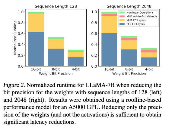
  • 이 문제를 더 자세히 설명하기 위해, 우리는 간단한 roofline 기반 성능 모델링 접근법(Kim et al., 2023)을 사용하여,
    A5000 GPU에서 다양한 bit precision으로 LLaMA-7B의 runtime을 연구함. (Fig 2)
    

  • 모든 computation이 FP16에서 유지된다고 가정하더라도, bit precision을 줄일수록 latency가 선형적으로 감소하는 것을 볼 수 있음.
    이는 주요 bottleneck이 compute가 아닌 memory임을 나타냄.

• 요약하면, 생성형 LLM inference에서 weight를 memory에 loading하는 것이 주요 bottleneck이며,
  dequantization과 FP16 computation의 비용은 상대적으로 작음.

  • 따라서, activation은 full precision으로 유지한 채
    weight만 lower precision으로 quantizing함으로써,
    상당한 speedup과 함께 model size 감소를 얻을 수 있음.

  • 이러한 insight를 바탕으로, 전략은 arithmetic operation에 overhead를 추가하더라도 memory size를 최소화하는 것.

Method

1. Sensitivity-based Non-uniform Q

• LLM의 weight distribution은 non-uniform pattern을 가짐.
  

• SqueezeLLM이 non-uniform Q를 선택한 이유

  • uniform Q의 두 가지 main issue

    • 1.LLM의 weight distribution은 non-uniform patterns

    • 2.uniform Q의 main 이점은 efficient integer computation인 반면, memory bound한 end-to-end latency를 향상시키진 않음.

• non-uniform Q의 optimal config를 찾는 것은 결국
  "k-means problem"을 푸는 것과 같다.

  • weight distribution이 주어졌을 때,
    목표는 $k$ 개의 centroid를 결정하는 것. (e.g., $k$=8 for 3-bit)

  • formulation of "optimization problem for non-uniform Q"
    

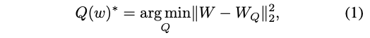
    • $W_Q$: quantized weights, represented by $k$ distinct values $\{q_1, ..., q_k\}$

  • optimal solution $Q(w)^*$는 1D k-means clustering으로 구할 수 있다.
    (parameter들을 k개의 cluster로 묶고, 각 cluster의 centroid를 q_j로 할당.)

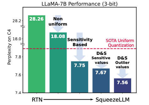
• 이 방법은 이미 uniform Q보다 성능이 좋지만,
  본 연구에서는 더 향상된 sensitivity-based clustering 알고리즘을 제안.

⭐ Sensitivity-Based K-means Clustering

• Quantization의 목표는 model weight를 low-bit precision으로 표현하면서 model output의 변화(perturbation)를 최소화하는 것.
  

• Quantization은 각 layer마다 perturbation을 일으키지만,
  각각의 layer에 focus하기 보단,
  final loss에 관한 overall perturbation을 최소화해야 한다.
  (Q 이후의 end-to-end 성능 하락에 더 direct한 measure)이기 때문.

  • 따라서, k-means centroid를 final loss에 관해 더욱 sensitive한 value 근처에 위치시켜야 한다.

• $\textcolor{red}{approximation \ 1}$
  더욱 sensitive한 value를 결정하기 위해,
  weights $W$의 변화(perturbation)에 따른 loss의 변화를
  Taylor expansion을 사용해서 $\textcolor{red}{approximation}$.
  
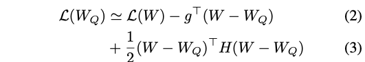
  $g = \frac{\partial{L(W)}}{\partial{W}}$ = gradient, $H = \mathbb{E}[\frac{\partial^2{L(W)}}{\partial{W^2}}]$ = hessian

• model이 converged 됐다고 가정하면, gradient $g \approx 0$
  $\therefore$ weights $W$의 변화(perturbation)에 따른 loss의 변화는 다음과 같다.
  (즉, 새롭게 정의된 optimization problem은 다음과 같다.)
  

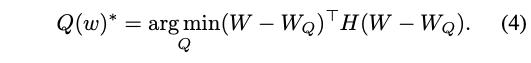
  • perturbation of each weight after Q, i.e. $W-W_Q$에
    scaling factor로 second-order derivative $H$가 곱해지는(weighted되는) 꼴이다.
  • 따라서, 큰 Hessian 값을 가진 weight들에 대한 변화(perturbation)를 최소화하는 것이 중요하다!!!

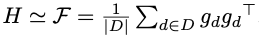
• $\textcolor{red}{approximation \ 2}$: Hessian을 Fisher info로 approx.

  • Hessian $H$를 computing하는건 비싸므로,
    Hessian을 Fisher information ${F}$를 기반으로 $\textcolor{red}{approximation}$.
    

  • 단지 일련의 sample에 대한 gradient를 계산하면됨.

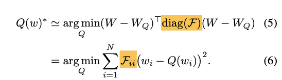
• $\textcolor{red}{approximation \ 3}$: Fisher info에서 diagonal만 사용.

  • Fisher information matrix에서 diagonal matrix만 사용.

  • diagonal(weight themselves)이 아닌(weight 간의 interaction)은 무시할만 한다고 가정.

  • 

• Eq (5)의 중요한 결론은 이 문제가 weighted k-means clustering 문제로 해석될 수 있다는 점.

  • centroid들은 sensitive한 weight 값들에 더 가깝게 끌려감.

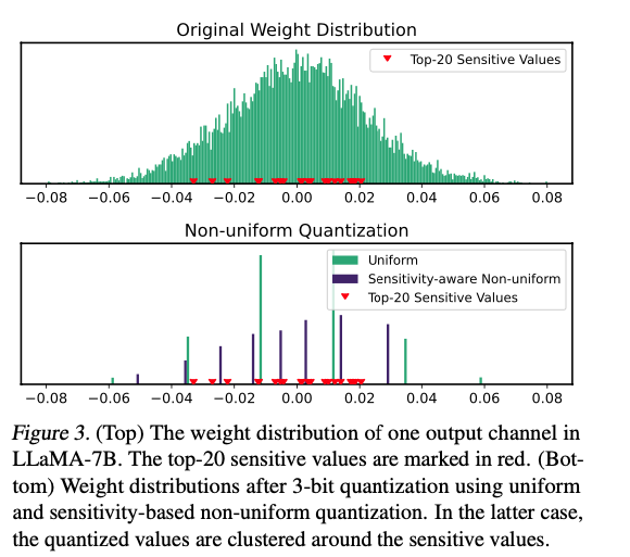
• Fig 3에서는 예시로 든 weight distribution의 Fisher information을 기반으로 상위 20개의 sensitive value를 보임.

  • 
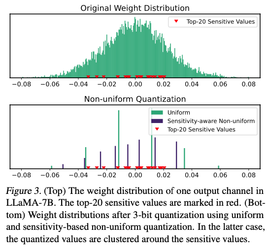
  • Sensitivity-based 접근법은 centroid를 sensitive value 근처에 배치함으로써 더 나은 trade-off를 달성하며, 이를 통해 quantization error를 효과적으로 최소화.
    

---

2. Dense-and-Sparse Q

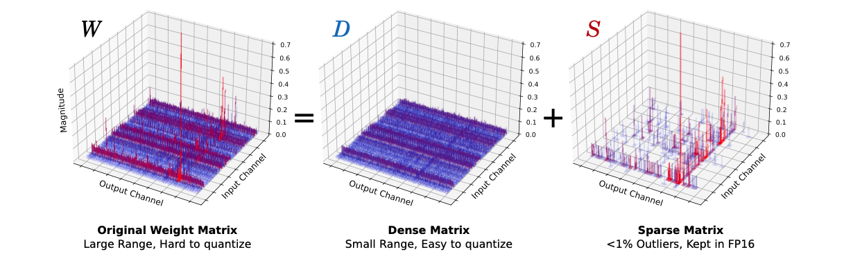
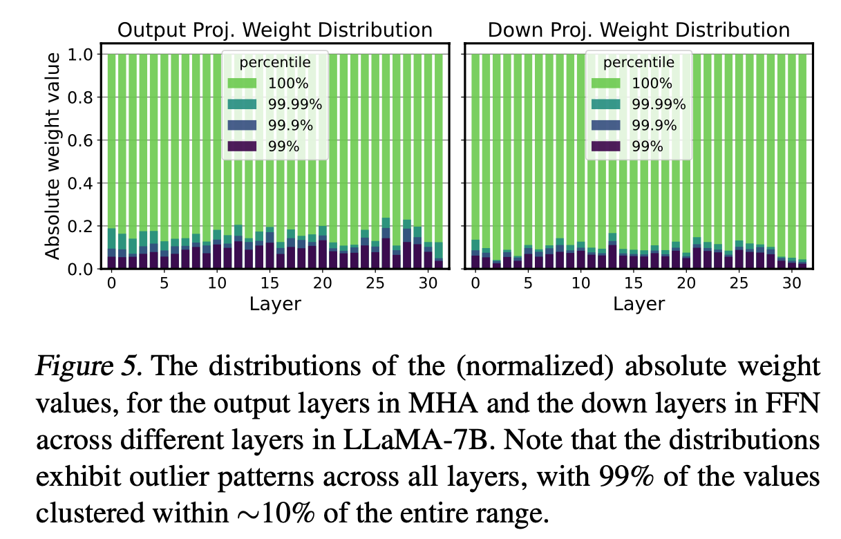
• weight의 ~99.9%는 전체 range의 ~10% 범위에 집중되서 분포.

  • 

  • 따라서, 단순히 weight를 Q하면, 성능 심각하게 하락.

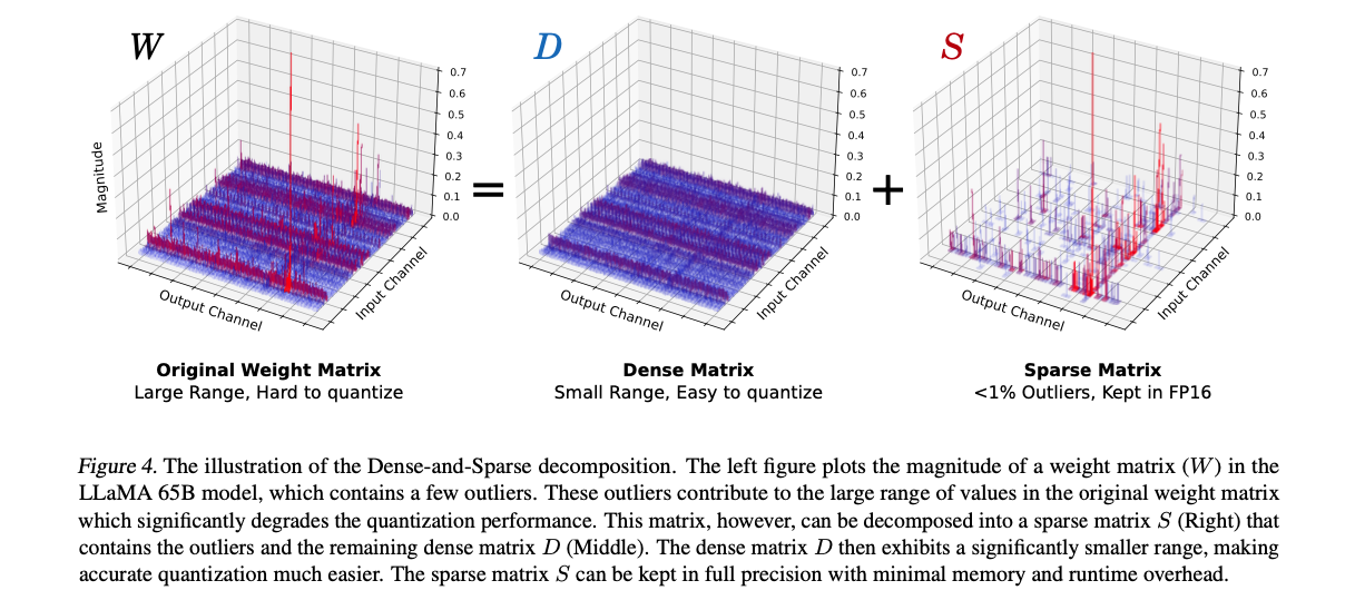
  • 하지만 이는 기회이기도 함.
    소수의 outlier value (예를 들어, 0.1%)만 제거함으로써
    weight value의 범위를 10배 정도 축소 가능.

    • 이는 quantization resolution 개선 가능.
    • 이는 sensitivity-based k-means의 centroid들이 소수의 outlier보다는 sensitive value들에 더 집중할 수 있도록 도와줌.

• weight matrix $W$를 S와 D로 decomposition

  • $W = D + S$

  • sparse matrix(S)

    • outlier 포함.
    • $S = W[w < T_{min}, \text{or}, w > T_{max}]$

  • dense matrix(D)

    • 나머지.
    • $D = W[T_{min} <= w <= T_{max} ]$

  • $T_{min/max}$는 distribution의 percentile을 토대로,
    outlier를 정하는 threshold.

• 

• 중요한 점은 이 decomposition의 overhead가 최소라는 점.

  • 이는 outlier value의 수가 적기 때문(예: 전체 value의 0.5%).
  • 따라서 sparse matrix는 compressed sparse row (CSR) 형식과 같은 방법을 사용하여 효율적으로 저장 가능.
  • Inference 또한 이 decomposition을 통해 간단해짐.
  • WX = DX + SX 형태로, dense와 sparse multiplication을 위한 두 kernel을 오버랩 가능.

Sensitivity-Based Sparse Matrix

• Outlier를 sparse matrix로 분리하는 것 외에도,
  소수의 highly sensitive한 weight matrix value를 정확하게 표현하는 것의 이점을 발견.
  
• sensitive한 value는 Fisher information을 기반으로 쉽게 식별했음.
• sensitive value들을 FP16으로 유지하여
  • 1) model output에 미치는 영향을 방지할 뿐만 아니라,
  • 2) Eq. 5의 centroid들이 sensitive value들로 치우치는 것을 막아줌.
    • Sensitive value들을 sparse matrix로 분리함으로써, 이 값들은 k-means clustering 과정에서 제외됨.
    • 결과적으로, 남은 weight들에 대해 더 균형 잡힌 clustering이 가능해짐.
    • 이는 centroid들이 극단적인 값들에 과도하게 영향받지 않고, 전체 분포를 더 잘 대표할 수 있게함.
• layer 전체에서 단 0.05%의 sensitive value들만 추출해도 quantization 성능을 상당히 향상시킬 수 있음을 관찰함.

---

GPTQ와의 차이점

• difference 1

  • SqueezeLLM: minimize the perturbation to the end layer

  • GPTQ try to minimize the perturbation not to the end layer, but to the specific layer that is being quantized.

  • Optimal Brain Damage [1] (which minimizes perturbations to the end layer/loss and is also used by our method)
    vs
    Optimal Brain Surgeon [4] (which minimizes perturbations to a specific layer in isolation and used by methods such as GPTQ).

  • This is expected since perturbation errors in a particular layer may not be important if the predictions of the network are not sensitive to that particular layer. (squeezeLLM authors)